graph LR
    Yt2["Y(t-2)"] --> Yt1
    Yt2 --> Yt
    Yt1["Y(t-1)"] --> Yt
    Yt1 --> Ytp["Y(t+1)"]
    Yt["Y(t*)"] --> Ytp

    D[Intervention] --> Yt
    D --> Ytp

    linkStyle 5,6 stroke:#F18F01,stroke-width:2px;
11 Time series methods: Measuring impact without a control group
Keywords
A/B Testing, Causal Inference, Causal Time Series Analysis, Data Science, Difference-in-Differences, Directed Acyclic Graphs, Econometrics, Impact Evaluation, Instrumental Variables, Heterogeneous Treatment Effects, Potential Outcomes, Power Analysis, Sample Size Calculation, Python and R Programming, Randomized Experiments, Regression Discontinuity, Treatment Effects
11.1 Play the hand you’re dealt
This chapter shows how to estimate causal effects when a conventional control group is unavailable but we can rely on historical data from the treated unit, which we call a time series.2 This is the only chapter focused on such methods, commonly known as Interrupted Time Series (ITS) analysis, which are essential when you lack a viable control group.
A word of caution: experimental methods and the quasi-experimental methods from previous chapters rely on control groups. We don’t have that luxury here. Instead, we take a different approach: we rely entirely on history. We use the treated unit’s past to predict its future, betting that, without the intervention, the old patterns would have continued.
Yet in practice these methods are often our only way to measure impact. This is particularly common in tech, where product changes and campaigns sometimes roll out platform-wide. For instance, when we roll out a new pricing model to all customers simultaneously, we lose the traditional control group but we may still want to learn about its causal effect.3
Before we dive in, a practical gut check: if you have untreated control units — other markets, regions, or comparable groups your intervention didn’t touch — Difference-in-Differences (Chapter 9) or Synthetic Control may be stronger choices. They leverage cross-sectional comparison rather than requiring a single series’ past to predict its future. This chapter is for the scenario where history is all you have, and ideally, a long, stable one (100+ periods).
The core idea is to use the metric’s history to predict what would have happened without the intervention. The gap between this prediction and the actual outcome is the estimated effect. Only by building this “synthetic” baseline can we measure impact when a parallel control group is missing.
This connects directly to the potential outcomes framework we learned in Chapter 2. In that language, our prediction serves as the counterfactual. Therefore, the treatment effect at time \(t\) is simply:
\[ \text{impact}_t = \text{Outcome}_{t,1} - \text{Outcome}_{t,0} \tag{11.1}\]
where \(\text{Outcome}_{t,1}\) is the observed outcome at time \(t\), and \(\text{Outcome}_{t,0}\) is the counterfactual (the outcome without treatment) which is not observable as we discussed in Chapter 2. As ITS uses historical data before the intervention to predict what the outcome would have been without the intervention, in the real-world case, Equation 11.1 becomes:
\[ \widehat{\mathrm{impact}}_t = \text{Observed outcome}_{t} - \text{Predicted outcome}_{t} \tag{11.2}\]
To generate this “Predicted outcome,” we rely on time series techniques, which is a field of its own. Stationarity, integration, and decomposition deserve their own deep dive, as they provide the necessary rigor for time series analysis — but that would take us far beyond this book’s scope.
Appendix 11.A offers brief explanations of these and other concepts, but if you plan to use the methods presented in this chapter often, I recommend building those fundamentals first. For approachable guides, see Hyndman and Athanasopoulos (2021) (R) and Hyndman et al. (2025) (Python). With that in mind, let’s explore the intuition behind the methods we’ll use here.
11.1.1 Intuition behind time series causal inference
“Prediction is very difficult, especially about the future.” — Attributed to Niels Bohr (Danish physicist, Nobel laureate)
Let’s make this concrete. You’re a marketing scientist tasked with estimating the impact of a national TV campaign (treatment) on sales (outcome). The campaign reaches all customers at once; no control group. You have access to historical data on sales before and after the campaign.
Before diving into the analysis, let’s preview the final output. Figure 11.1 illustrates this. The solid black line tracks actual sales before and after the campaign. The dashed vertical line marks the intervention. The dashed blue line is the counterfactual — predicted sales if the campaign hadn’t happened. Before the intervention, both lines nearly overlap, as expected: no campaign, no effect.
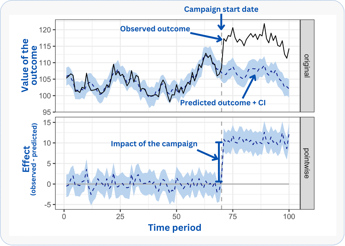
The challenge: estimating the blue dashed line after the intervention. We’re asking: what would sales have been without the campaign? This is what matters because the difference between this counterfactual scenario and the actual sales we observed is the causal effect we are trying to measure.
CausalImpact and Causal ARIMA (C-ARIMA for short) construct this counterfactual using pre-intervention data. Both can incorporate auxiliary series (related metrics like organic search traffic, weather data, or industry indices that correlate with your outcome but were not affected by the intervention) though they do so in different ways (Brodersen et al. 2015; Menchetti, Cipollini, and Mealli 2023). By modeling the pre-intervention behavior of the treated series, these methods project its likely path into the post-intervention period, effectively creating a synthetic counterfactual.
In Figure 11.1, focus on the top panel: notice how closely the counterfactual (blue) tracks the observed (black) before the intervention. This alignment is your sanity check, as the model should fit the pre-period well. After the intervention, the gap that opens up is your estimated lift. The bottom panel isolates this gap, showing magnitude and statistical significance (does the confidence band exclude zero?).
But this counterfactual’s credibility depends on a few assumptions we’ll explain when we discuss C-ARIMA (Section 11.2.1). For now, keep three ideas in mind: (1) the intervention should be persistent and the only major shock to affect the outcome variable, (2) historical patterns of your time series should persist, and (3) there should be no anticipation effects. Violate these, and your counterfactual becomes unreliable.
As we dive into C-ARIMA and CausalImpact, we’ll explore each method’s specific assumptions. But one practical implication cuts across all of them: counterfactual accuracy degrades over time.
The further you project into the post-intervention period, the less reliable your counterfactual becomes. Prediction uncertainty grows as we move away from known data, and unmodeled external events become more likely to disrupt historical patterns.
A 2-week estimate is more trustworthy than a 2-month one. When possible, keep your analysis window short: just long enough to capture the effect, but not so long that unmodeled changes accumulate.
With those practical guideposts in mind, let’s clarify what we’re actually estimating.
11.1.2 What causal estimands are we estimating?
When a campaign affects your entire business, you’re asking: “How much did this help or hurt us?” Imagine you launch a marketing campaign on March 1st that targets all your users. There’s no control group because everyone sees the campaign. The only way to measure its impact is to compare:
- What actually happened to your sales after March 1st: your observed business path
- What would have happened to your sales if you hadn’t run the campaign: your counterfactual business path
The difference between these two is your campaign’s effect. Note that cross-sectional terminology doesn’t map perfectly to time series settings. If we view the business as a single unit (N=1), we are technically estimating an Individual Treatment Effect (ITE).
However, if we see this single time series as an aggregation of many treated units (buyers in a marketplace), it effectively captures the Average Treatment Effect on the Treated (ATT). I use ATT here to clarify that we are measuring the realized impact on the specific group that received the intervention (e.g. your business) rather than a hypothetical Average Treatment Effect (ATE) on the entire market.
In formal terminology, this difference at each time point is called the point effect. We can then aggregate point effects into a cumulative effect (sum over time) or a temporal average effect (mean over time) (Menchetti, Cipollini, and Mealli 2023).
But since you’re estimating the effect on your specific business (or platform, or market), be cautious about extrapolating. The ATT tells you what happened here, not what would happen elsewhere. For generalization, you’d need theory, additional data, or experiments in other contexts.
One technicality worth flagging: cumulative effects only make sense for flow metrics — quantities measured over an interval, like daily sales, sign-ups, or clicks. For stock metrics — quantities defined at a point in time, like total active users or account balance — cumulative effects are uninterpretable (Brodersen et al. 2015).
If your campaign adds 100 new users on day 1 and 50 on day 2, the cumulative effect (150 new users) makes sense. But if you’re measuring total active users (a stock), summing daily values is meaningless — you’d be double-counting. For stock metrics, report only the point effect or the temporal average effect.
11.2 Causal ARIMA: time series meets potential outcomes
Causal ARIMA (C-ARIMA) repurposes the well-established ARIMA framework for causal inference when a traditional control unit is unavailable (Menchetti, Cipollini, and Mealli 2023). Before diving into the causal aspects, let’s briefly understand what ARIMA models are and why they matter for our purpose.
To use ARIMA for causality, we first need to understand it as a pattern-recognition machine.
The autoregressive (‘AR’) component captures autocorrelation: the tendency of today’s value to depend on yesterday’s. If your app had 10,000 daily active users yesterday, you won’t have 100,000 today or 1,000 tomorrow. Business metrics are sticky — they don’t jump randomly. The ‘p’ in ARIMA(p,d,q) tells us how many past days the model should remember when predicting the next one.
The integrated (‘I’) component handles trends. Maybe your user base is growing steadily at 2% per month. ARIMA handles this by “differencing” the data, looking at day-to-day changes rather than absolute values. The ‘d’ parameter tells us how many times to apply this differencing to achieve stationarity, meaning the average and variability of your metric settle into a predictable pattern rather than drifting.
The moving average (‘MA’) component is the most subtle. It says that today’s surprise (the error in yesterday’s prediction) contains information about tomorrow. If we underestimated yesterday’s sales by 20%, that error itself becomes useful information. The ‘q’ parameter determines how many past surprises we remember.
Here’s a concrete example: your e-commerce platform’s daily revenue follows an ARIMA(1,1,1) model. Today’s revenue depends on yesterday’s (AR=1), we need to difference once to remove the growth trend (I=1), and yesterday’s prediction error helps adjust today’s forecast (MA=1). In plain English: revenue is sticky day-to-day, it’s growing over time, and when we’re wrong, we learn from it.
Caveat: differencing removes linear trends (steady growth of X units per day), but it won’t fix all non-stationarity issues. If your series has structural breaks (sudden level shifts), exponential growth patterns, or volatility that changes over time, differencing may not be enough. The residual diagnostics we’ll discuss later check for leftover autocorrelation, but they don’t directly test whether the series is stationary. If you suspect deeper issues — say, your pre-intervention data contains a major disruption like a product pivot or market shock — consider truncating the data to exclude the unstable period.
Here’s where it gets interesting. C-ARIMA repurposes this forecasting machinery for causal inference, and the way it does so is what makes it causal rather than just predictive. The key design choice: C-ARIMA estimates all parameters exclusively from pre-intervention data. It never sees post-intervention outcomes during training. This is what separates it from traditional regression-with-ARIMA-errors (REG-ARIMA), which estimates on the full series including post-intervention periods and therefore cannot cleanly distinguish “what would have happened” from “what did happen.”
By fitting only on the “before” period, C-ARIMA constructs an honest counterfactual: “Based on what I learned from January and February, here’s what March and April would have looked like if nothing had changed.” The gap between this projection and the observed outcome is the estimated causal effect (Equation 11.2). This clean separation between training data (pre-intervention) and evaluation data (post-intervention), combined with the potential outcomes framework and assumptions described below, is what gives C-ARIMA its causal interpretation (Menchetti, Cipollini, and Mealli 2023).
11.2.1 What needs to be true for C-ARIMA to work?
Before applying C-ARIMA, we must discuss assumptions. These aren’t just technical checkboxes; they’re the foundation of whether your causal claims will hold. Menchetti, Cipollini, and Mealli (2023) formalize three core assumptions (3.1-3.3). I’ve expanded these into practical rules that include both their formal requirements and additional guardrails from experience. Some of these expand on what we listed in Section 11.1.1.
1. The “single persistent intervention” rule
Menchetti, Cipollini, and Mealli (2023) call this Assumption 3.1: once treatment turns on at time \(t^*\), it stays on for all subsequent periods. The intervention is a clear-cut event that splits time into “before” and “after,” and the definition of treatment is unambiguous throughout.
In practice, many interventions are transitory — marketing campaigns end, special offers expire. The formal assumption is stronger (treatment is irreversible), but the pragmatic interpretation is this: treatment must be strictly on throughout the window you’re analyzing. A campaign that ran for 3 weeks and then stopped is fine; just define your post-intervention period as those 3 weeks. Do not extend the window into the period where the treatment was turned off, or the “before vs. after” distinction breaks down.4
What goes wrong if violated: If your intervention flickers on and off (e.g., you turn a feature on for a week, off for a week, then on again) within your analysis window, the definition of “after” becomes ambiguous. The model cannot estimate a stable effect because the treatment condition itself is unstable.
How to check: Review release logs or activity metrics to confirm when treatment started and whether it stopped or paused. Define your post-intervention period to cover only the period where treatment was continuously active. (Note that this windowing strategy is a common practical adaptation — the formal proofs in Menchetti, Cipollini, and Mealli (2023) assume permanent, irreversible intervention.)
1b. The “no concurrent shocks” requirement
This is a separate identification concern from treatment persistence. Formally, a concurrent shock violates Conditional Stationarity (Assumption 3.3): the data-generating process changes for reasons unrelated to your intervention. I list it as its own rule because practitioners encounter it as a distinct, recognizable threat. Without a control group, C-ARIMA cannot separate your intervention’s effect from other simultaneous changes. The only “shock” that should hit your outcome series at time \(t^*\) is your intervention.5
What goes wrong if violated: If a competitor exits the market the same week you launch a campaign, sales will rise. C-ARIMA sees this jump and attributes all of it to your campaign and none to the fact that you just coincidentally gained market share.
How to check: Detective work, not a statistical test. Maintain a rigorous event log. Check for other marketing launches, product changes, or external news events that coincide with your intervention window.
2. The “stable patterns” rule
The cornerstone assumption: the series’ pre-intervention behavior (trends, seasonality, autocorrelation) would have continued unchanged without the intervention. We are essentially betting that the “rules” governing your metric didn’t change right when you launched your campaign.
Formally, this is conditional stationarity (Menchetti, Cipollini, and Mealli 2023). Technically, this stationarity condition applies to the untreated potential outcome \(Y(0)\) — the series that would have been observed absent the intervention. In plain terms: the “rules” connecting yesterday’s values to today’s predictions must stay the same across your entire dataset. This is what allows us to learn patterns from observed pre-period data and project them forward to predict the unobserved counterfactual \(Y(0)\) in the post-period — the period where we never get to see what would have happened without the intervention.
What goes wrong if violated: Imagine analyzing sales data that’s been stable for years. Just as you launch your campaign, a global recession hits. The “rules” of consumer spending change fundamentally. Your model, trained on pre-recession data, predicts high sales, but actual sales are low because of the recession. The difference is negative, and you might conclude your campaign caused the drop — when it was the recession.
How to check: Visually inspect pre-intervention data for structural breaks — moments when underlying patterns fundamentally changed (new competitor, pandemic, etc.). Also watch for sudden shifts in volatility. Statistical tests like the Chow test can help detect these breaks formally. If your pre-period contains major disruptions (e.g., the start of COVID-19), consider truncating the data or explicitly modeling those shifts.6
3. The “no anticipation” rule
The outcome shouldn’t react to the intervention before it actually happens. Users can’t change behavior in anticipation of a campaign they don’t know about. Menchetti, Cipollini, and Mealli (2023) state this explicitly: there should be no anticipatory effects in the data. Interestingly, they point out that no-anticipation is actually implicit in the conditional stationarity assumption: if the intervention affected outcomes before \(t^*\), the data-generating process would have changed, violating stationarity.7
What goes wrong if violated: If users learn about a sale before it officially launches (through leaks, pre-announcement buzz, or internal communication), they may delay purchases to wait for the discount. The pre-intervention data shows an artificial dip, which the model treats as the “normal” trajectory and projects forward. After the sale launches, the bounce-back looks like a huge effect, but part of it is just pent-up demand that was always going to materialize.
How to check: Inspect the days immediately before the intervention. Is there an unusual dip or spike that looks like anticipatory behavior? Also, consider whether the intervention was publicly announced before it went live. Secret launches are cleaner for causal inference than widely publicized ones.
4. The “unaffected covariates” rule
C-ARIMA can include external predictors via its xreg parameter — for example, weather data, holiday indicators, or market indices (Menchetti, Cipollini, and Mealli 2023, Assumption 3.2). If you use such covariates, they must be independent of your intervention.
What goes wrong if violated: Suppose you use “competitor price” as a predictor. You lower your price (the intervention), and competitors immediately react by lowering theirs. If you include their price in your model, the model will attribute the change in sales to the competitor’s price drop, not your intervention. You “control away” your own effect.
How to check: Run a causal analysis on the predictor itself. Does your intervention appear to “cause” a change in the predictor? If so, either drop it or (if the covariate is essential) substitute its counterfactual values in the post-period. Menchetti, Cipollini, and Mealli (2023) do exactly this in their supermarket application: when a store-brand price cut directly changed the product’s unit price, they replaced post-intervention prices with what the price would have been without the discount, preserving the covariate’s predictive value without contamination.
C-ARIMA’s xreg support means the method is not limited to univariate analysis. The CausalArima() function accepts external regressors in both R and Python, learning their relationship with the outcome during the pre-intervention period and using their post-intervention values to sharpen the counterfactual forecast. See Appendix 11.B for a worked example comparing C-ARIMA with and without external regressors.
Don’t dismiss covariates as optional extras. In many real-world settings, external regressors are what make the “stable patterns” assumption (Conditional Stationarity) plausible in the first place. Menchetti, Cipollini, and Mealli (2023)’s own empirical application relied on holidays, day-of-week dummies, and price data. Without these, the raw series would have shown patterns shifting for reasons unrelated to the intervention, violating the very foundation of the method.
5. The “enough history” rule
ARIMA can overfit when trained on short series. If your pre-period is too brief, the model may capture noise as signal, producing overconfident predictions.
What goes wrong if violated: Your counterfactual looks precise (narrow confidence bands) but is actually unreliable. The model “memorized” quirks in your limited data rather than learning generalizable patterns.
How to check: Perform out-of-sample validation: split your pre-period, train on the first half, predict the second. If forecast errors are large, your time series may be too short or too noisy for reliable causal inference.
11.2.2 Visualizing C-ARIMA’s causal structure
A DAG (directed acyclic graph) helps visualize which causal relationships C-ARIMA assumes exist (arrows) and which it assumes do not exist (missing arrows). Figure 11.2 shows the temporal structure underlying this method. Read the diagram left to right: time flows from pre-intervention to post-intervention. Each node represents the outcome at a point in time; the orange node \(D\) is our intervention.
The diagram captures C-ARIMA’s core logic. The arrows \(Y_{t-2} \rightarrow Y_{t-1} \rightarrow Y_t \rightarrow \dots\) represent the autoregressive structure: \(Y_{t-1}\) feeds into \(Y_{t*}\), and because this is AR(2), \(Y_{t-2}\) also directly affects \(Y_{t*}\), in addition to its indirect influence through \(Y_{t-1}\). This is the “AR” in ARIMA. The arrow from \(D\) to \(Y_{t*}\) shows the intervention affecting outcomes starting at time \(t^*\).
What the diagram doesn’t show matters just as much. There is no arrow from \(D\) to \(Y_{t-1}\) — this is the no anticipation assumption. Users can’t change behavior before they know about the intervention. There is also no common cause connecting \(D\) and \(Y\) that isn’t accounted for by temporal patterns — we assume the intervention timing is exogenous, not driven by the outcome itself.
11.2.3 Practical implementation of C-ARIMA
before we write a line of code, let’s map out C-ARIMA’s three-step logic (Menchetti, Cipollini, and Mealli 2023). It is simple:
Estimate on pre-intervention data only. Fit an ARIMA model to the data before the intervention. This learns the historical patterns, the relationship with any external variables, and the specific noise level of your data. Post-intervention data is never seen during training.
Forecast the counterfactual. Using the estimated parameters, project what \(Y\) would have been at each future date if the intervention hadn’t happened. This is a standard long-range forecast, extended with external variables if you included them.
Compute the causal effect. At each post-intervention day, subtract the forecast from the observed value. This is Equation 11.2 in action: \(\text{Effect} = \text{Actual} - \text{Predicted}\). This gives a time series of effects — not one number, but a trajectory showing how the impact evolved day by day.
From these point effects, you can derive three estimands: the cumulative effect (sum of daily effects — total impact so far), the temporal average effect (cumulative divided by number of days — average daily lift), and in multi-unit settings, the cross-sectional average (average across units at each time point).
Let’s implement C-ARIMA step-by-step using a realistic business scenario.
TipWant to run the code? Set up your environment: click here
Data: All data we’ll use are available in the repository. You can download it there or load it directly by passing the raw URL to read.csv() in R or pd.read_csv() in Python.8
Packages: To run the code yourself, you’ll need a few tools. The block below loads them for you. Quick tip: you only need to install these packages once, but you must load them every time you start a new session in R or Python.
# Install CRAN packages (run once)
# install.packages(c("tidyverse", "forecast", "CausalImpact", "devtools"))

# Install CausalArima from GitHub (run once)
# devtools::install_github("FMenchetti/CausalArima")

# Load packages (run every session)
library(tidyverse)    # Data manipulation and visualization
library(forecast)     # Time series forecasting tools
library(CausalImpact) # Bayesian causal inference for time series
library(CausalArima)  # Causal ARIMA implementation
library(gridExtra)    # Visualization tools
# pip install pandas matplotlib causalimpact statsmodels scipy
# pip install git+https://github.com/RobsonTigre/pycausalarima.git
# Core packages
import pandas as pd # Data manipulation
import matplotlib.pyplot as plt # Visualization
from pycausalarima import CausalArima # Causal ARIMA implementation
from causalimpact import CausalImpact # Bayesian causal inference
# Diagnostic packages (used in robustness checks)
from statsmodels.stats.diagnostic import acorr_ljungbox
from statsmodels.graphics.tsaplots import plot_acf, plot_pacf
from scipy.stats import shapiroLet’s implement C-ARIMA using simulated data to measure the impact of a national marketing campaign on daily e-commerce sales, with day-of-week seasonality.
This data mirrors realistic business scenarios, and since I created it, I know the true effect: +R$ 20 MM/day in sales. Figure 11.3 shows our sales time series. Before reading on, notice: (1) the regular up-and-down pattern — Saturdays peak around R$155-160 MM, Mondays dip to R$120-130 MM (weekly seasonality); (2) after day 85, the series shifts upward by ~R$20 MM. This visual jump is what we’re trying to quantify.
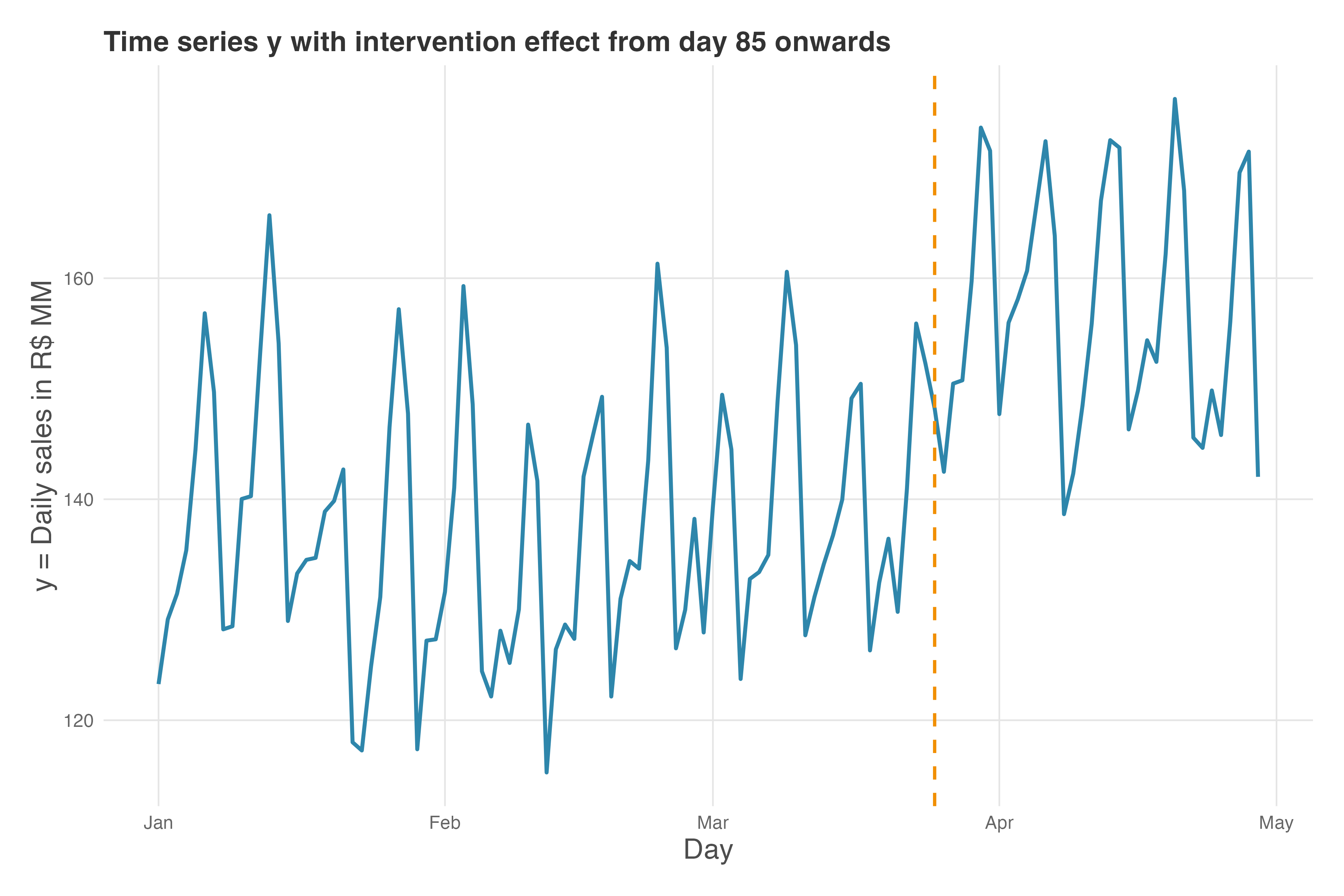
Sales rise and fall by day of the week, mimicking the seasonality in most real high-frequency data. In our example, Saturdays and Sundays have higher baseline sales, while Mondays are lower, meaning that certain days (or weeks, or months) consistently behave differently, often due to business cycles, customer habits, or operational factors.9
After the intervention, sales are clearly higher. This is what we need to estimate — accounting for seasonality. Here’s how, in both R and Python.
Figure 11.4 shows the C-ARIMA counterfactual forecast. The black line tracks observed sales; the blue dashed line with shaded confidence band is the model’s prediction of what would have happened without the campaign. Before the intervention (vertical dashed line), the forecast closely tracks the observed data — as expected, since there’s no treatment effect yet. After day 85, the observed values consistently exceed the forecast. This gap is the estimated causal effect.
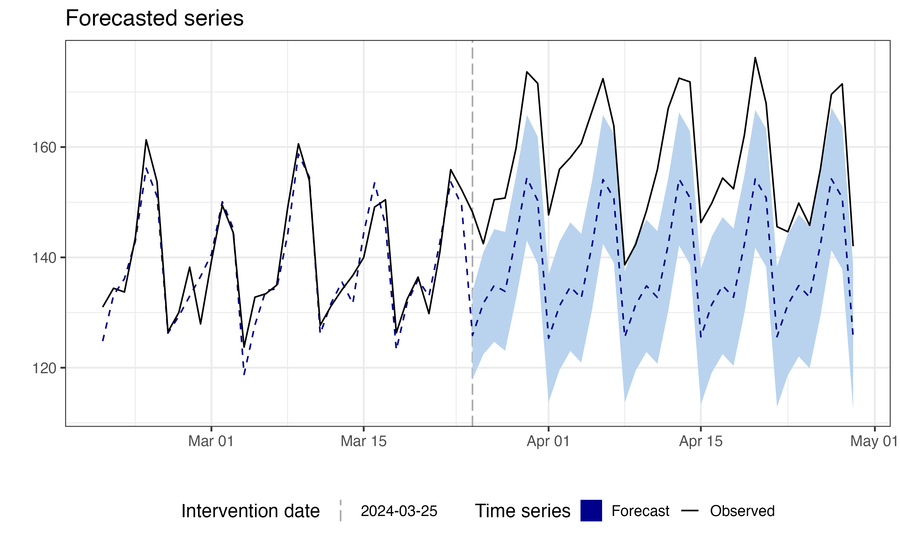
Under the assumptions discussed earlier, comparing forecast to actual post-intervention data isolates the causal effect — valuable when no control group exists. To calculate confidence intervals and p-values, the model uses bootstrap techniques, providing flexibility and robustness in the estimates.10
The impact() function returns the estimated causal effect. C-ARIMA automatically selected an ARIMA(2,0,0)(2,1,0)[7] model in R — today depends on the last 2 days, with seasonal patterns repeating every 7 days.11 (If this notation looks cryptic, Appendix 11.A has a full decoder.) The key results, mapped to the estimands from step 3 above:
- Temporal average effect: R$ 18.5 MM/day (95% CI excludes zero, p < 0.001) — the average daily lift across the 36-day post-period
- Cumulative effect over 36 days: R$ 666 MM — the total impact accumulated since intervention (36 × 18.5 = 666)
This R$ 18.5 MM/day estimate is remarkably close to the true R$ 20 MM/day (only ~7.5% underestimation). Later, I’ll show how CausalImpact, which leverages auxiliary data through its Bayesian state-space framework, gets even closer to the true value by incorporating additional signals into its counterfactual.
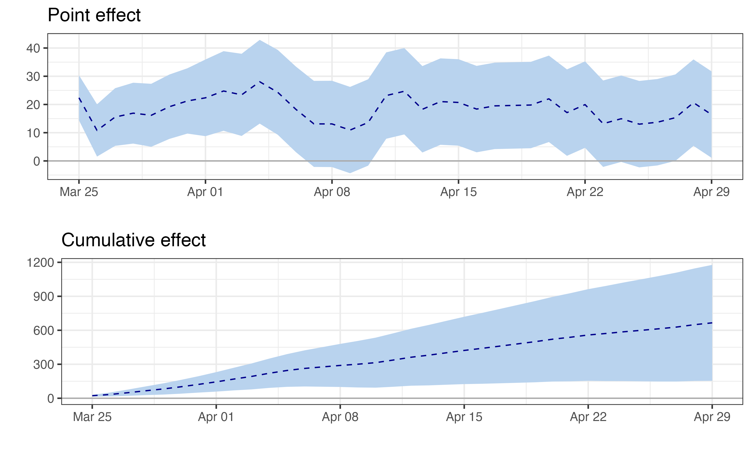
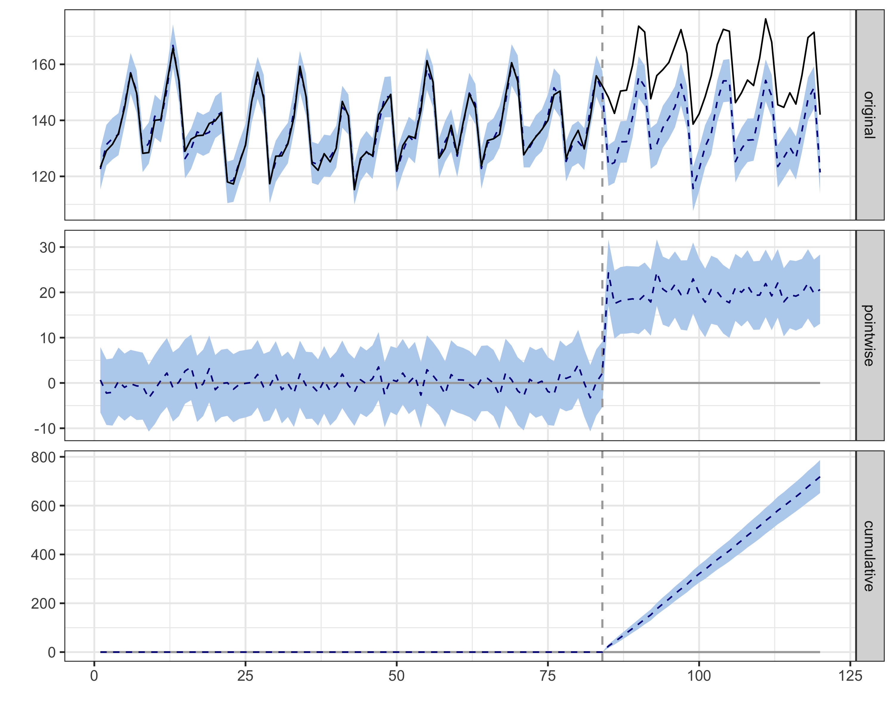
Figure 11.5 shows the estimated impact over time. The top panel shows the pointwise effect (observed minus predicted) for each day — daily impact fluctuates around R$18-19 MM, with 95% CIs remaining above zero. The bottom panel shows the cumulative effect building steadily toward R$665-680 MM. Notice how the confidence bands exclude zero throughout — strong evidence that the campaign had a real, sustained effect.
Here, daily impact appears stable. But in real campaigns, effects often decay — novelty wears off, customers habituate, competitors respond. If daily impact shrinks toward zero, that’s not model failure; it’s the effect genuinely fading. When reporting, distinguish peak effect (largest daily impact), sustained effect (impact in final days), and cumulative effect (total over the period). A campaign with a huge early spike that fades to zero may have a large cumulative effect but no lasting business impact.
You might be wondering: “Why not just fit a regression with ARIMA errors and add a dummy variable for the post-intervention period?” This traditional approach (REG-ARIMA) is common but has subtle risks — specifically, it struggles to detect effects that aren’t constant level shifts (like a gradual ramp-up or a temporary spike). C-ARIMA avoids this by estimating a time series of point effects rather than a single average coefficient. For a detailed comparison of why REG-ARIMA can mislead you — and the simulations that prove it — see Appendix 11.C.
11.2.4 Robustness check: do your results hold up under placebo?
As we discussed before, we need several assumptions to hold before we can claim causality, some of which are not directly testable. The placebo test is one way to check for violations of these assumptions.
Menchetti, Cipollini, and Mealli (2023) emphasize residual diagnostics as the primary model validation tool (we cover those in the next section), while Brodersen et al. (2015) frame a similar exercise as prospective power analysis.
I lead with the placebo test because I find it more intuitive for practitioners and convincing to stakeholders.12 The principle is simple: a sound method shouldn’t find effects where none exist. Like testing a metal detector in your backyard before hitting the beach — if it beeps constantly in your garden, something’s wrong.
Pick a date before your actual intervention and pretend the campaign launched then. Run C-ARIMA on this fake scenario. If it finds a significant effect during this pre-period, you have a problem. Your model is either overfitting to noise, picking up some pattern you haven’t accounted for, or there’s something else happening in your data.
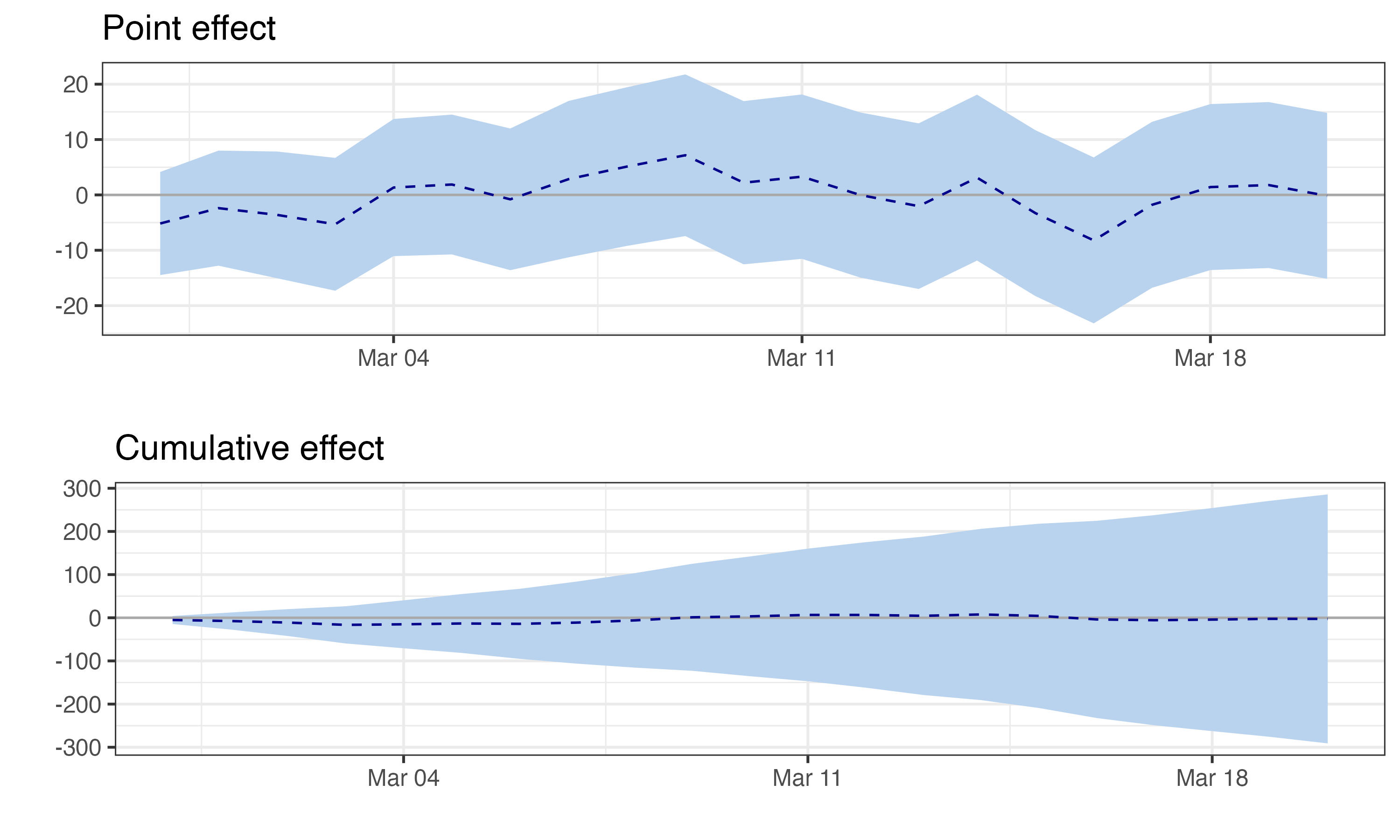
The placebo results are reassuring: the estimated average effect is R$ -0.1 MM/day — essentially zero — with p = 0.95. Well above the 0.05 threshold, so we fail to reject the null of no effect. In plain terms: when we pretend the campaign started 25 days earlier than it did, the model correctly finds nothing. This gives us confidence the significant effect at the real intervention date isn’t spurious.
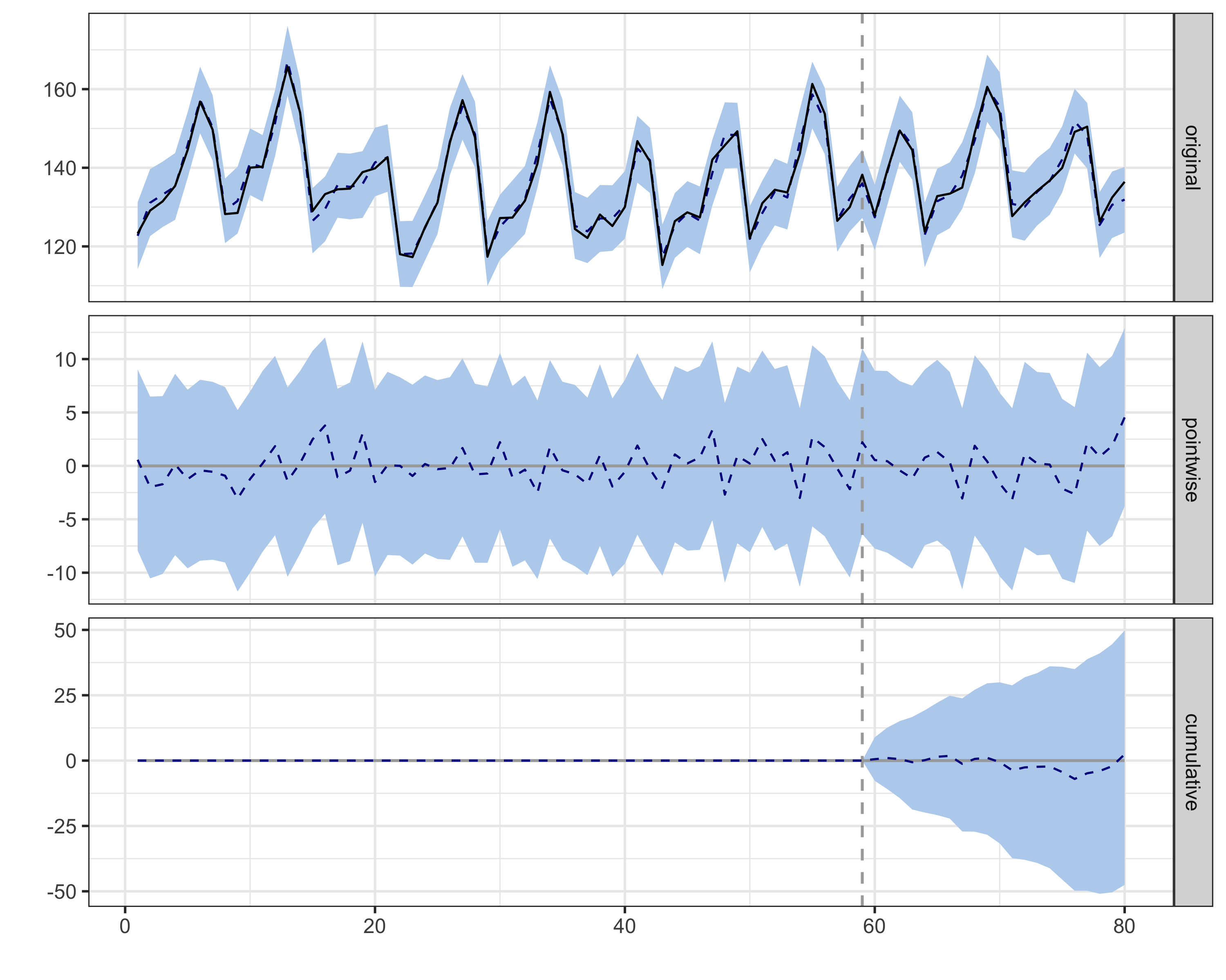
Figure 11.6 shows the placebo impact estimates. Notice how the confidence bands comfortably include zero throughout the fake post-period — exactly what we want to see. Takeaway: If this test had found a significant effect, we’d know our model was picking up noise or confounding trends, casting doubt on our main results.
11.2.5 Robustness check: are the model residuals well-behaved?
The placebo test checks whether the model finds effects where none should exist. But there’s another important validation: checking whether the ARIMA model itself is correctly specified. If the model is misspecified (wrong order, missing seasonality, structural breaks), the counterfactual forecast will be biased — and so will your causal estimate.
The key diagnostic is residual analysis. If the ARIMA model has captured all the predictable structure in your data, the residuals (prediction errors) should look like random noise — no patterns, no autocorrelation. If you see patterns in the residuals, the model missed something.
We’ll use three complementary diagnostics:
Ljung-Box test: This is a formal statistical test for autocorrelation in the residuals. The null hypothesis is that the residuals are independently distributed — in other words, that knowing today’s error tells you nothing about tomorrow’s. If the model captured all the predictable structure, errors should be as random as coin flips. A high p-value (above 0.05) means we fail to reject that null — good news, because it suggests no leftover autocorrelation.
Shapiro-Wilk test: This tests whether residuals are normally distributed. Normal residuals are consistent with a well-specified model — they suggest the ARIMA structure left behind only random noise — but this check complements, rather than replaces, the autocorrelation diagnostics above.
There’s a practical bonus, too: Menchetti, Cipollini, and Mealli (2023) offer two inference strategies, analytic and bootstrap confidence intervals. The analytic path (their Theorem 4.1) requires Gaussian errors — when that holds, the effect estimator is also Gaussian, so standard errors and p-values follow directly without simulation.
The bootstrap path makes no distributional assumptions, and the
CausalArimapackage uses it by default, so normality isn’t strictly required for valid inference. But when the Shapiro-Wilk test confirms normality, the faster analytic CIs become available as a cross-check. A high p-value (above 0.05) means we can’t reject normality.
ACF and PACF plots: These visualize autocorrelation at different time lags. The ACF (autocorrelation function) shows the correlation between a residual and residuals at earlier times. The PACF (partial autocorrelation function) shows the direct correlation after removing the influence of intermediate lags.
In both plots, the shaded band represents the 95% confidence interval under the null hypothesis of no autocorrelation. If bars extend beyond this band at any lag, the model missed a pattern at that lag. For a well-specified model, no significant spikes should appear beyond lag 0.
For more on these diagnostics, see the appendix to this chapter.
In our example, the residual diagnostics are clean:
Ljung-Box test: p = 0.99 (R) / 0.64 (Python).13 Since these are well above 0.05, we fail to reject the null hypothesis of no autocorrelation. The residuals appear to be independently distributed — the model hasn’t left predictable structure on the table. Conclusion: The ARIMA specification is adequate; there’s no evidence that adding more AR or MA terms would improve the counterfactual forecast.
Shapiro-Wilk test: p = 0.10 (R) / 0.96 (Python). Again, well above 0.05, so we cannot reject the null hypothesis that residuals are normally distributed. Since the bootstrap CIs used by C-ARIMA are distribution-free, this test isn’t strictly necessary for valid inference — but it’s still informative. Normal residuals indicate good model fit, and they also mean you could use the faster analytic CIs from Menchetti, Cipollini, and Mealli (2023) (Theorem 4.1) as a cross-check. Conclusion: Residuals look well-behaved, which supports the overall model specification.
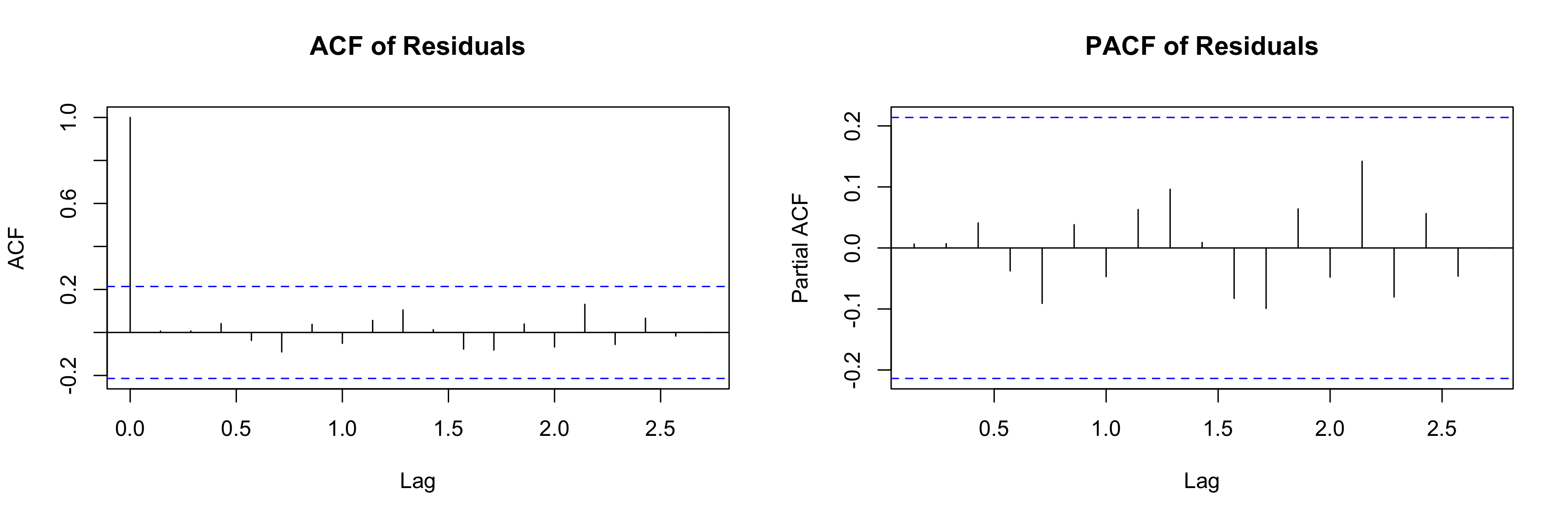
- ACF/PACF plots (Figure 11.7): These plots show whether residuals at different time lags are correlated with each other. No significant spikes beyond lag 0 means the residuals look like random noise — exactly what we want. This visual confirmation matches what the Ljung-Box test told us statistically. Conclusion: No missed seasonality or lagged dependencies — the model captured the temporal structure in the data.
Together, these diagnostics suggest the ARIMA model is well-specified. The counterfactual forecast is built on solid ground, which gives us more confidence in our causal estimate.
11.2.6 Bridging the gap: C-ARIMA can use covariates too
We ran C-ARIMA without auxiliary series, but as mentioned earlier, it can and should incorporate them through its xreg parameter. So if both methods accept auxiliary variables, what’s the real distinction?
This analogy captures the default usage of each method. C-ARIMA is like a seasoned e-commerce analyst who has memorized your sales patterns — she knows Saturdays peak, Mondays dip, and holiday weeks spike. If you hand her a report on organic search traffic, she’ll use it, but her forecast is primarily built from the sales rhythm she already knows. The auxiliary data refines her prediction at the margins.
CausalImpact is more like a market analyst who monitors an entire dashboard of signals — organic search, competitor pricing, industry indices — and synthesizes them into a view of “what normal looks like.” Its architecture is designed to leverage these auxiliary series as a core component of the counterfactual, not an afterthought. It automatically determines which variables matter (via spike-and-slab priors — a Bayesian model averaging technique that averages over all possible subsets of predictors, weighting each by how well it explains the data) and can even allow their coefficients to evolve over time.
They trade off different risks; understanding how they use auxiliary data differently will help you interpret results and choose wisely. The decision framework later in this chapter (Section 11.4.3.4) lays out when each method shines. Let’s now see how CausalImpact works. (For a worked example of C-ARIMA with external regressors, see Appendix 11.B.)
11.3 CausalImpact: a structural Bayesian time series approach
Developed by Google researchers (Brodersen et al. 2015), it uses a Bayesian Structural Time Series (BSTS) model that incorporates auxiliary series — like organic search traffic or industry indices — as additional evidence for what “normal” looks like.14
Auxiliary series help triangulate the truth. Back to our marketing campaign. Using sales alone would be risky — what if there was an economic shift we hadn’t captured? Instead, include related metrics the campaign shouldn’t have affected: industry-wide trends, weather, or unrelated indicators (stock market, exchange rates).15
The beauty is in how CausalImpact uses this information. During the pre-intervention period, it learns the contemporaneous relationships: “When organic search traffic is up 10% on a given day, sales tend to be 3% higher that same day.” “When competitor prices are 5% higher today, our sales are typically 3% higher today.” It’s building a model of how your business ecosystem moves together, day by day.16
Then comes the clever part. After your marketing campaign, CausalImpact observes what happened to all these auxiliary series and asks: “Given that organic traffic stayed flat and competitor prices dropped 2%, what would sales have done without the marketing campaign?” It’s like having a much more sophisticated baseline that accounts for the complex web of factors affecting your business.17
Figure 11.8 shows our auxiliary series \(x_1\) alongside the intervention marker. Notice how \(x_1\) fluctuates around a stable mean of approximately 55 throughout the entire period — it shows no structural break when the campaign launches. This is exactly what we need: a series that captures general business conditions (the “weather” of your market) without being contaminated by your intervention. In our simulated data, \(x_1\) represents something like organic search traffic or a market index that correlates with sales but isn’t directly affected by the TV campaign.
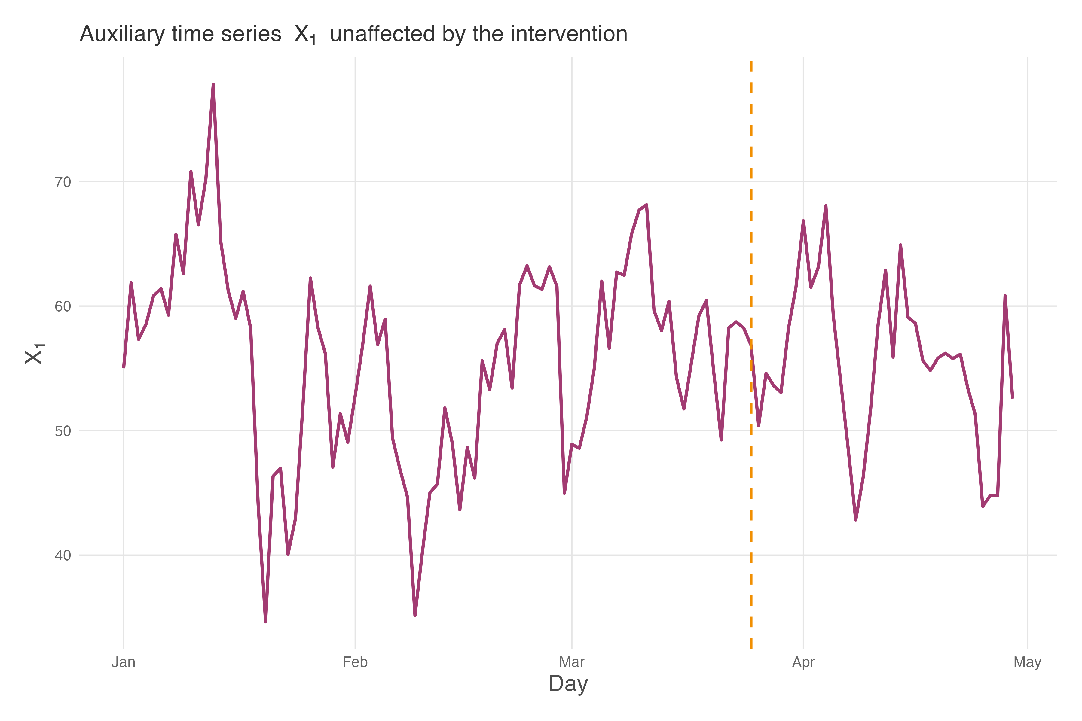
The logic of CausalImpact works like this: during the pre-intervention period (days 1-84), the model learns that sales (\(y\)) and \(x_1\) tend to move together. When \(x_1\) goes up, sales typically go up too. After the intervention, CausalImpact observes what actually happened to \(x_1\) and asks: “Given that \(x_1\) followed this particular path, what should sales have been if the campaign had no effect?” The difference between this prediction and actual sales is the estimated causal effect. By anchoring the counterfactual to an unaffected auxiliary series, CausalImpact produces a more credible estimate than methods that rely solely on temporal patterns.
11.3.1 What needs to be true for CausalImpact to work?
Brodersen et al. (2015) state their assumptions clearly throughout the paper but do not consolidate them into a numbered checklist the way Menchetti, Cipollini, and Mealli (2023) do. The rules below gather those stated requirements into one place and add practical diagnostic guidance. CausalImpact’s strength is that auxiliary data is a structural part of the model through its Bayesian state-space framework, not a supplement. But this strength creates new vulnerabilities.
When run without covariates, C-ARIMA needs nothing else to change (the “no concurrent shocks” requirement). CausalImpact can partially relax this: other things can change, as long as your auxiliary series capture them. C-ARIMA with external regressors can also absorb some shared variation, but CausalImpact’s Bayesian state-space framework is more flexible at this. The trade-off is real, though — if your auxiliary series are contaminated by the intervention, CausalImpact will bias your estimate downward, potentially performing worse than C-ARIMA without covariates (Brodersen et al. 2015). The flexibility comes with its own strict rules.
1. The “stable relationship” rule
This is similar to C-ARIMA’s “stable patterns” rule, but with an important addition. While C-ARIMA assumes that the history of your metric predicts its future (e.g., “sales always dip on Mondays”), CausalImpact also assumes that the relationship between your metric and the auxiliary series remains constant (e.g., “when organic search rises, sales rise”).
There are two levels of stability to think about:
Parameter stability. This doesn’t mean coefficients must be frozen in time. In fact, one of CausalImpact’s strengths is that it allows them to drift gradually. Think of it like a river slowly changing course: that’s natural. What breaks the assumption is the river suddenly jumping to a new channel overnight.
In practical terms: if the relationship “organic search drives 3% of sales” has slowly shifted to 4% over the past year, the model can handle it. But if that relationship abruptly jumps to 10% on the day your campaign launches, the model’s counterfactual will be wrong. The way the parameters drift must remain consistent pre- and post-intervention.
Structural stability. This means the functional form of the model itself stays constant. The trend remains linear, the seasonality remains weekly, and the set of relevant variables doesn’t change. Brodersen et al. (2015) warn that “all preceding results are based on the assumption that the model structure remains intact throughout the modelling period.” Their simulations show that when structure breaks — for example, if the volatility of the trend suddenly triples after the intervention — estimation errors explode.
What goes wrong if violated: If the relationship breaks, your counterfactual becomes fiction. Suppose Google updates its algorithm during your campaign, making organic search less predictive of sales. The model, unaware of this structural break, keeps applying the old rule. It predicts sales based on a relationship that no longer exists, leading to a biased estimate.
How to check: This is hard to test directly because you can’t observe the counterfactual relationship. However, you can check for stability in the pre-period. Split your pre-intervention data into two halves and train the model on the first half to predict the second. If it fails to predict the pre-intervention data accurately, the relationship is likely unstable or the model is misspecified.
2. The “unaffected auxiliary series” rule
This is the most important — and most common — failure mode. Your auxiliary series must be a valid control — meaning it must be completely unaffected by your intervention. It should be a witness to the “business weather,” not a participant in your campaign. In other words, we may say that there is no spillover effect from one series to the other and the auxiliary series is not affected by the intervention.
What goes wrong if violated: If your intervention lifts the auxiliary series, CausalImpact will interpret that lift as “normal market conditions” and predict that your sales should have gone up too. It effectively “controls away” your impact.
Recall the example where you use organic search as a control for a paid ad campaign. If your ads increase brand awareness, driving more people to search organically, your control is contaminated. The model sees organic search rising and thinks, “Oh, interest is high naturally, so sales would have been high anyway.” It subtracts this “natural” increase from your actual sales, shrinking your estimated effect.
How to check: Run a CausalImpact analysis on the auxiliary series itself. Treat the auxiliary series as the outcome (\(y\)) and see if your intervention had a significant effect on it. If it did, you cannot use it as a control.
But being unaffected is necessary, not sufficient. An auxiliary series must pass two tests: (1) it wasn’t affected by your intervention, and (2) it actually predicts your outcome well. A series that’s clearly unaffected but uncorrelated with sales — like stock prices of an unrelated company — adds no information. It’s like having a witness who wasn’t at the crime scene and can’t remember anything useful. Before including an auxiliary series, check its correlation with your outcome in the pre-period. If the correlation is weak (say, below 0.3), the series won’t help CausalImpact build a better counterfactual, even if it passes the “unaffected” test.
4. The “sufficient history” rule
CausalImpact is a Bayesian method. This means it starts with a prior belief about the world and updates it with data. If you have very little data (short pre-intervention period), the data can’t speak loudly enough to override the prior.
What goes wrong if violated: With insufficient data, your result basically reflects your prior assumptions, not the reality of the data. The model might produce extremely wide credible intervals (saying “the effect is between -50% and +50%”), or worse, it might converge on a nonsensical answer driven by default settings.
How to check: There is no magic number for “enough data,” but a good heuristic is to ensure your pre-period covers several cycles of the seasonality you want to model. If you have weekly seasonality, you need many weeks of data. If the credible intervals in your results are so wide they are useless for decision-making, you likely don’t have enough pre-intervention data to constrain the model.
5. The “no anticipation” rule
Just as with C-ARIMA, the outcome should not react to the intervention before it actually happens. If users change behavior in anticipation of a campaign they haven’t yet seen, the pre-intervention data is contaminated, and the counterfactual built from it will be biased. The same checks from C-ARIMA’s “no anticipation” rule (Rule 3 above) apply: inspect the days immediately before the intervention for unusual dips or spikes, and consider whether the intervention was publicly announced before it went live.
6. The “quality over quantity” rule
A natural concern: what if your auxiliary series are highly correlated with each other? In traditional regression, this multicollinearity makes coefficient estimates unstable. But CausalImpact’s spike-and-slab prior (described in the previous section) was designed precisely for this scenario. This Bayesian model averaging approach can handle “tens or hundreds of potential variables” (as the authors note), so you don’t need to manually prune correlated series the way you would in OLS.
That said, throwing in every available series is not free. Extreme collinearity among many weak predictors can slow MCMC convergence or produce wider credible intervals without improving the counterfactual. And every additional series introduces the risk of violating the “unaffected auxiliary” rule above, which is a far bigger threat than collinearity.
How to choose well: Focus on two questions for each candidate series: (1) Was it unaffected by the intervention? (2) Does it genuinely predict the outcome in the pre-period? If both answers are yes, include it and let the spike-and-slab prior handle redundancy. If you have dozens of candidates and worry about computational cost, prioritize series with the highest pre-period correlation to your outcome.
11.3.2 Bayesian inference: quantifying uncertainty
CausalImpact is built on Bayesian Structural Time-Series (BSTS) models. Think of BSTS as a flexible forecasting engine that decomposes your metric into components (trend, seasonality, and the influence of related metrics) while honestly tracking how uncertain each component is.19 But how is it different from just running a regression as we learned in Chapter 1?
Look, traditional methods give you a point estimate plus a confidence interval: “The campaign increased sales by 15% (95% CI: 10%-20%).” But what does that interval mean? In the frequentist view, it’s a statement about hypothetical repetitions — “if we repeated this experiment many times, 95% of intervals constructed this way would contain the true effect.” Awkward, right? Bayesian inference asks a more natural question: “Given what we observed, what’s the probability distribution of possible effects?” The result is a credible interval you can interpret directly.
This matters a lot for decision-making. There’s a world of difference between an interval of “15% ± 2%” (i.e., 13% to 17%) and another of “15% ± 20%” (i.e., -5% to 35%). The first suggests high precision; the second screams “we’re not really sure!”. CausalImpact quantifies this uncertainty by running thousands of simulations, each one a plausible version of what might have happened without your intervention. This technique (called Markov Chain Monte Carlo, or MCMC, if you want to impress someone at a conference) maps out the full range of counterfactual possibilities, not just a single best guess.
The practical upshot: when CausalImpact says “there’s a 95% probability your true effect lies between 10% and 20%”, you can interpret this literally, provided the model is correctly specified. Unlike traditional confidence intervals (which technically make claims about repeated experiments, not your specific case), Bayesian credible intervals directly answer the question you actually care about: “What’s the likely range of my intervention’s true effect?” For a business stakeholder, this clarity is gold. (For more on credible intervals and MCMC, see the appendix to this chapter.)
There’s another practical advantage: automatic variable selection. In real analyses, you might have dozens of potential control series — organic search, email clicks, competitor prices, weather data, stock market indices. Which ones should you include? Traditional approaches force you to choose manually, risking both overfitting (too many variables) and omitted variable bias (too few).
CausalImpact automatically figures out which auxiliary variables actually help predict your outcome. Variables that add no predictive value get effectively ignored; useful ones get weighted according to their contribution. (The spike-and-slab prior handles this by averaging over variable combinations to filter out noise. See Brodersen et al. (2015) for the technical details.) You don’t have to agonize over variable selection; the model does it for you, while honestly accounting for the uncertainty in that selection.
11.3.3 Visualizing CausalImpact’s causal structure
Like C-ARIMA, CausalImpact is fundamentally a time series method — it relies on temporal patterns to build the counterfactual. But it adds a powerful ingredient: auxiliary series that help predict the outcome. Figure 11.9 shows this structure, deliberately paralleling the C-ARIMA DAG to highlight what’s similar and what’s different. Solid arrows represent causal or temporal relationships. Dashed arrows represent predictive relationships — \(X\) helps predict \(Y\) but doesn’t necessarily cause it.
graph LR
    Xt1["X(t-1)"] --> Xt["X(t*)"] --> Xtp["X(t+1)"]
    Yt1["Y(t-1)"] --> Yt["Y(t*)"] --> Ytp["Y(t+1)"]
    Xt1 --> Yt1
    Xt --> Yt
    Xtp --> Ytp
    D[Intervention] --> Yt
    D --> Ytp

    linkStyle 7,8 stroke:#F18F01,stroke-width:2px;
Compare this to the C-ARIMA DAG (Figure 11.2). Both share the horizontal arrows showing temporal evolution. But there’s a subtle difference in how temporal dependence works under the hood. In C-ARIMA, past outcomes directly predict current outcomes (autoregression). In CausalImpact, temporal dependence flows through latent states — unobserved components like trend (\(\mu_t\)) and seasonality (\(\gamma_t\)) that evolve over time and generate the observed \(Y\) values (Brodersen et al. 2015). The \(Y \rightarrow Y\) arrows in the DAG are a simplification for exposition; more precisely, a latent state \(\alpha_t\) evolves from \(\alpha_{t-1}\), and each \(Y_t\) is generated from \(\alpha_t\) plus noise.20
What CausalImpact adds is the vertical relationship: auxiliary series \(X\) helping predict \(Y\) at each time point. Note that \(X\) need not cause \(Y\); CausalImpact only requires that \(X\) predicts \(Y\) without being affected by the intervention. The model learns this \(X \rightarrow Y\) relationship during the pre-intervention period and applies it during the post-intervention period to build a sharper counterfactual.
The critical assumption appears as an absence: there is no arrow from \(D\) to \(X\). The intervention affects only the \(Y\) series. If your marketing campaign boosted brand awareness, driving up organic search traffic, then \(D \rightarrow X\) would exist — and CausalImpact would attribute part of your campaign’s effect to “normal market conditions,” biasing your estimate downward. This is why the “unaffected auxiliary series” rule in Section 11.3.1 is non-negotiable.
11.3.4 Practical implementation of CausalImpact
Now let’s see CausalImpact in action using the same business scenario. The key difference from C-ARIMA? We’ll leverage an auxiliary series (x1) to build a sharper counterfactual.
The CausalImpact output is rich with information. The fundamental logic is the same as C-ARIMA: Effect = Actual - Predicted. Let’s unpack the key results:
Average causal effect: R$ 20 MM/day, with a 95% credible interval of [18, 22] MM/day. How to read this: we’re 95% confident the true daily effect falls somewhere in this range. This is remarkably close to the true effect of R$ 20 MM/day that we built into the simulation — and very close to C-ARIMA’s estimate of R$ 18.5 MM/day. Both methods converge on similar values, which is reassuring.
Cumulative effect: R$ 719 MM (R) / R$ 706 MM (Python) over the 36-day post-intervention period — the gap reflects differences in estimation methods across implementations.21
Relative effect: The campaign increased sales by approximately 15% [13%, 16%] relative to what they would have been without the intervention.
Posterior probability: 99.98%. CausalImpact is highly confident this effect is real, not a statistical fluke.
The summary(impact_ci, "report") function generates a plain-language interpretation that you can share directly with stakeholders. It states that “the positive effect observed during the intervention period is statistically significant and unlikely to be due to random fluctuations” — exactly what you need to justify the campaign’s ROI.
Notice how the inclusion of the auxiliary series \(x_1\) tightened our estimate. By leveraging information about how sales typically co-move with \(x_1\), CausalImpact built a more accurate counterfactual. This is the triangulation principle in action: multiple data sources converging on a more credible answer.
Figure 11.10 shows the CausalImpact output. The top panel displays observed sales (solid line) against the counterfactual prediction (dashed line with shaded credible interval). Before the intervention, the two lines track closely — the model fits the pre-period well. After day 85, the gap that opens up is our estimated effect. The middle panel isolates this pointwise effect over time, showing the daily lift hovering around R$20 MM with credible intervals consistently above zero. The bottom panel shows the cumulative effect building steadily toward ~R$710-720 MM. These are Bayesian credible intervals — you can interpret them literally.22
An important technical detail: CausalImpact does not generate independent predictions for each post-intervention day. Instead, it draws joint counterfactual trajectories — complete paths of what might have happened — preserving the connection between consecutive days (Brodersen et al. 2015). This is what makes the cumulative credible intervals in the bottom panel trustworthy: the uncertainty in the total effect accounts for the fact that tomorrow’s counterfactual is connected to today’s, rather than naively summing independent bounds.
Moreover, each trajectory is drawn from a different plausible version of the model — different parameter values, different combinations of auxiliary variables (weighted by the spike-and-slab prior we discussed in Rule 6) — so the final credible intervals reflect not just “how uncertain are we about the effect given our model” but also “how uncertain are we about which model is correct.” This Bayesian model averaging is what prevents CausalImpact from overfitting to a single specification (Brodersen et al. 2015).
11.3.5 Robustness checks for CausalImpact
The power of auxiliary series comes with a responsibility: more complexity means more ways things can go wrong. The same placebo framework we used for C-ARIMA applies, but now we can also test each auxiliary series.
Robustness check 1: Placebo test
We apply the same logic: pick a date before your intervention, pretend treatment happened then, and verify the model finds no effect.
The placebo test results are exactly what we hoped for:
- Estimated effect: ~0.1 MM/day (R) / ~0.8 MM/day (Python) — both indistinguishable from zero
- 95% credible interval: [-2.3, 2.4] (R) / [-4.5, 6.4] (Python), comfortably includes zero
- Posterior probability: p = 0.47 (R) / 0.36 (Python) — both indistinguishable from chance
CausalImpact’s auto-generated report states that “the effect is not statistically significant, and so cannot be meaningfully interpreted.” This is the correct conclusion when analyzing a fake intervention date. The model isn’t hallucinating effects where none exist, which gives us confidence that the significant effect we found at the real intervention date reflects genuine causality, not model artifacts.
Figure 11.11 shows these placebo results visually. Notice how the pointwise effect (middle panel) fluctuates around zero throughout the fake post-period, with credible intervals comfortably spanning zero. The cumulative effect (bottom panel) drifts randomly rather than building systematically. This is exactly what we want to see — no spurious signal at a date where no intervention occurred.
Robustness check 2: Was the auxiliary series affected?
This test validates the “unaffected auxiliary series” rule from Section 11.3.1. The logic is simple: run a causal analysis on the auxiliary series itself. If you find a significant effect at the intervention date, you cannot use that series as a control.
In our simulated data, we know that \(x_1\) was designed to be unaffected by the intervention — it’s a pure AR(1) process with trend that we generated independently. The C-ARIMA analysis on \(x_1\) confirms this: the estimated average daily effect on \(x_1\) is approximately R$ -0.4 MM (95% CI includes zero, p = 0.89) — no statistically significant structural break at the intervention date. The counterfactual forecast for \(x_1\) tracks the actual values closely in the post-period.
This is exactly what we need to validate CausalImpact’s key assumption. If you were analyzing real data and found that your auxiliary series was affected by the intervention, you would need to either find a different control variable or acknowledge that your CausalImpact estimate may be biased.
Sensitivity analysis: How much does the auxiliary series matter?
CausalImpact can run with or without covariates. This sensitivity check asks: “How much does our estimate depend on the auxiliary series?” If results are similar with and without x1, your estimate is robust. If they differ substantially, you should carefully validate that x1 is a good predictor and truly unaffected by the intervention.
The comparison reveals something important:
| Metric | With \(x_1\) | Without \(x_1\) |
|---|---|---|
| Average effect | R$ 20 MM/day | R$ 19.5 MM/day |
| 95% CI | [18, 22] | [17, 22] |
| Relative effect | 15% | 14% |
Both estimates are very close — with or without \(x_1\), we get ~R$ 19-20 MM/day. This suggests our estimate is robust: the auxiliary series adds precision but doesn’t dramatically change the point estimate. Both methods (C-ARIMA at R$ 18.5 MM and CausalImpact at R$ 20 MM) converge on similar values, close to the true effect of R$ 20 MM/day.
The similarity between the with-\(x_1\) and without-\(x_1\) estimates is actually good news — it means our result isn’t overly dependent on the auxiliary series. But what if the estimates had diverged dramatically — say, from R$ 20 MM to R$ 5 MM? That’s a signal to investigate further. Either the auxiliary series is adding valuable information that corrects a biased estimate, or it’s contaminated by the intervention and biasing the result downward. The robustness check in the previous section helps distinguish between these scenarios.
By now, you’ve seen the power of these methods and the importance of robustness checks. But before you rush off to apply them to every business question, we need to have an honest conversation about what these methods can’t do — because knowing what a tool can’t do is just as useful as knowing what it can.
11.4 The honest conversation: what these methods can’t do
11.4.1 Aggregation issues and individual-level effects
Aggregation hides information. When we roll up individual user actions into daily metrics, we flatten the heterogeneity of human behavior. Let me illustrate with a hypothetical scenario.
A team launches a new recommendation algorithm. Their time series analysis declares a rousing success — 5% lift in overall engagement! Champagne is popped. Bonuses are discussed. Then a junior analyst segments the analysis by user tenure.
The reality is stunning: new users (less than 7 days old) show a 40% increase in engagement. But power users — the ones who’ve been around for years — show a 10% decrease. They hate the change. Since power users make up 70% of daily active users, the aggregate 5% increase is actually a weighted average of triumph and disaster.
The fundamental problem: time series methods treat your user base as a monolith. But users aren’t a monolith. They’re individuals with different needs, behaviors, and responses to change.
Worse: temporal cannibalization. I’ve seen campaigns that increased daily revenue (success!) but decreased weekly revenue (failure!). The campaign pulled forward purchases that would have happened anyway. Day-by-day, it looked great. Week-by-week, it was cannibalizing future sales.
Aggregation can also create Simpson’s paradox23 — where a positive effect within each customer segment somehow becomes negative overall. This happens when the intervention shifts who is buying. If a discount attracts more price-sensitive customers (who spend less per order), the campaign might boost sales in every segment while lowering average order value overall.
So what can you do? First, acknowledge the limitation. When you report results, be clear: “This is the average effect across all users.” Second, supplement with segmented analyses whenever possible. Even if you can’t run causal analysis on each segment, at least look at the raw trends. Third, track compositional metrics. If your intervention changes who uses your product, not just how much they use it, you need to know.
11.4.2 General limitations of time series causal inference
The fundamental identification challenge
To be brutally honest: time series causal inference is built on a heroic assumption — that the future resembles the past. When we use historical data to predict a counterfactual, we’re essentially saying, “The world would have continued on its current trajectory if not for our intervention.”
As we noted in Section 11.1.1, counterfactual accuracy degrades over time. It’s like weather forecasting: tomorrow’s prediction is pretty good, next week’s is questionable, and next month’s is basically guesswork.
This lesson can be painful. Imagine evaluating a pricing change that shows fantastic results over two weeks. Management wants to wait for a full month of data to “be sure.” By week four, a competitor launches a major campaign, the economy hiccups, and your beautiful causal estimate becomes meaningless. The world has changed too much.
Unobserved confounders remain problematic
Here’s what keeps me up at night: the things we don’t know we don’t know. Time series methods can only account for what we measure. But in the complex ecosystem of digital business, unmeasured forces are always at play.
Your competitor’s CEO decides to slash prices but hasn’t announced it yet. Apple changes App Store ranking algorithms without telling anyone. A social media influencer randomly mentions your product. These events happen constantly, and time series methods will blindly attribute their effects to your intervention.
The only defense is paranoia — healthy, productive paranoia. Document everything. Track competitor actions obsessively. Monitor social media mentions. Build dashboards for metrics you don’t even care about, because they might matter someday. The confounder that ruins your analysis is always the one you didn’t think to measure.
Model uncertainty compounds over time
When CausalImpact gives you a credible interval, it’s being honest — but only partially. That interval accounts for parameter uncertainty given the model, but what about uncertainty in the model itself? Should you use 7-day seasonality or 7 and 30-day? Which auxiliary series should you include? How long should your pre-period be?
Each choice affects your results, sometimes dramatically. I’ve seen estimated effects swing from significantly positive to significantly negative just by changing the pre-intervention period by two weeks. Yet the model’s uncertainty estimates don’t capture this model selection uncertainty.
The implication is sobering: our uncertainty bands are lower bounds on true uncertainty. The real uncertainty is always greater — sometimes much greater — than what our models report.
11.4.3 A decision framework for these methods
So, we have powerful tools with serious limitations. How do you decide when to proceed? After years of applying these methods, I’ve developed a simple decision framework — a “go/no-go” gauge for the pragmatic data scientist.
Green lights: use ITS confidently
These methods are your best friend when you have a platform-wide change with no holdout group — the classic scenario where A/B testing is impossible. But to replace a control group, you need history on your side. These models use pre-intervention data extensively — learning from the past to predict the future. Within CausalImpact’s Bayesian framework, this learning combines prior beliefs about plausible parameter values with the observed data; with 100+ days of history, the data dominates and default priors work well. With a stable history of at least 100 days, the model can grasp your metric’s “personality” and confidently project it forward.
The situation gets better if you have powerful auxiliary series. Think of these as your control group in spirit, if not in practice. If you have data on a similar market or a related metric that your intervention didn’t touch, both CausalImpact and C-ARIMA (via xreg) can use it to triangulate the counterfactual — though CausalImpact’s automatic variable selection makes it the more natural choice when you have many candidate series.
Finally, these methods shine when you need directional speed over decimal-point precision. If you need to know “did this roughly work?” in two days to make a rollout decision, you have a green light.
Here’s a lesser-known trick: you can use CausalImpact before your intervention for prospective power analysis (Brodersen et al. 2015). Pick a date in the past and pretend it was your intervention. Run the model and look at the width of the credible intervals. If the 95% interval spans ±15%, you know you won’t reliably detect effects smaller than that. This is essentially a power analysis — without the formulas.
To calibrate your expectations: Brodersen et al. (2015) ran 256 simulations and found that small effects (~1%) are missed the vast majority of the time, while only large, unambiguous effects are reliably detected (see their Figure 3b for the full power curve). The false positive rate under the null hypothesis was appropriately controlled at ~5%. The takeaway: CausalImpact is not a tool for detecting subtle effects. If your anticipated lift is modest, you have a substantial chance of missing it even if it’s real. You may need a very long pre-period, very strong auxiliary series, or a different method altogether. Run this simulation exercise before committing resources to a campaign that can’t be measured.
Yellow lights: proceed with extreme caution
Be very careful when the intervention is triggered by the outcome itself. This happens when you launch a campaign because sales are tanking. This is a feedback loop or reverse causality problem — treatment timing is driven by the outcome, which violates the exogeneity needed for causal identification. The problem is double-edged. First, things often bounce back naturally (regression to the mean). If you intervene right at the bottom, your model might count that natural operational recovery as a causal win, biasing your results upwards.
Second, and perhaps more subtly, you might underestimate the true effect. If your model assumes the metric would naturally recover (based on historical stability) when, in reality, it would have kept crashing without your help, you are in trouble. It is like giving medicine to the sickest patient in the hospital: even if the medicine works miracles and stabilizes them, they might still look unhealthy compared to the average person. If your counterfactual assumes “average health” instead of “continued decline,” your successful intervention might look like a failure.
Also, beware of sparse data. If you only have monthly data points, you are trying to paint a detailed portrait with a pixelated brush. You likely lack the granularity to detect subtle shifts unless the effect is massive. Proceed, but treat your results as broad hints rather than precise measurements.
Red lights: stop and reconsider
The biggest red light is having a better option. If you can run an A/B test, do it. No time series model can beat the internal validity of a randomized experiment. Similarly, if you have credible untreated control units, Difference-in-Differences (Chapter 9) or Synthetic Control will give you stronger identification than forecasting from a single series. Don’t use a sledgehammer when you have a scalpel.
You should also stop if your pre-intervention data is a roller coaster. Menchetti, Cipollini, and Mealli (2023) highlight that valid predictions usually require “stable patterns” (or patterns that become stable after simple transformations). If your metric was chaotic or structurally changing before your campaign (say, due to a competitor’s aggressive moves) you cannot reliably project that chaos forward. You are trying to predict a pattern that doesn’t exist.
Another deal-breaker is the “detective’s dilemma”: simultaneous interventions. If three different teams launch major features on the same Tuesday, and metrics spike, who takes credit? The model sees one big jump and has no way to disentangle which feature caused it. You have violated the “no concurrent shocks” requirement, and no amount of math can solve that forensic mystery.
Choosing between C-ARIMA and CausalImpact
Here’s a whiteboard-style breakdown of when each method earns its place in your analysis.
| Dimension | C-ARIMA | CausalImpact |
|---|---|---|
| Counterfactual engine | Y’s autoregressive structure (AR/MA/differencing) drives the forecast; X enters as fixed regression coefficients | Latent state-space model (trend + seasonality) plus X as a structural regression component |
| Variable selection | Manual — you choose which X to include | Automatic via spike-and-slab priors (Bayesian model averaging) |
| Coefficient behavior | Fixed across the entire series | Can be static or dynamic (time-varying via random walk) |
| Inference framework | Frequentist: Standard estimation + bootstrap CIs | Bayesian: posterior distribution + MCMC credible intervals |
| Causal framework | Explicit potential outcomes (Rubin Causal Model) | Counterfactual derived from the posterior predictive distribution |
Use C-ARIMA when:
- Your outcome has strong, well-understood autoregressive patterns (yesterday’s sales reliably predict today’s).
- You have few candidate auxiliary variables and know exactly which ones to include.
- You want an explicit connection to the potential outcomes framework and prefer frequentist inference.
- You suspect your auxiliary series might be weakly contaminated and prefer to rely on Y’s own history as the primary counterfactual driver.
Use CausalImpact when:
- You have many candidate auxiliary series and want the model to sort out which ones matter (automatic variable selection shines here).
- Your outcome’s own history is noisy or has weak autocorrelation, so auxiliary series add substantial predictive power.
- You want Bayesian uncertainty quantification — posterior probabilities and credible intervals that stakeholders can interpret directly.
- The relationship between X and Y may evolve over time, making dynamic regression coefficients valuable.
Run both when you can. If both methods agree on the direction and approximate magnitude, your estimate is robust. If they disagree substantially (say, C-ARIMA reports a +15% lift and CausalImpact reports +3%), that divergence is diagnostic. It signals that one of your assumptions is likely violated: perhaps the auxiliary series is contaminated (biasing CausalImpact downward), or a concurrent shock hit your outcome (biasing C-ARIMA upward). The disagreement itself is information.
11.5 Wrap up and next steps
We’ve covered a lot of ground. Here’s what we’ve learned:
- Prediction as counterfactual: When control groups are impossible, we bet on history. We use pre-intervention patterns to predict what would have happened without the intervention. The gap between prediction and reality is the estimated causal effect.
- Two complementary methods: C-ARIMA and CausalImpact both construct counterfactuals from pre-intervention data, but differ in how they use auxiliary information. C-ARIMA builds the counterfactual from the outcome’s own autoregressive structure and treats external regressors as supplements. CausalImpact makes auxiliary series a structural component of the model, with automatic variable selection via spike-and-slab priors.
- The price of entry: These methods demand strict conditions: a single persistent intervention (no flickering on and off), no concurrent shocks (or auxiliary series that capture them), stable pre-intervention patterns, unaffected covariates, and no anticipation effects. Violate any one, and your counterfactual becomes unreliable.
- Robustness is non-negotiable: Placebo tests, residual diagnostics, and auxiliary series contamination checks are not optional add-ons. They are your primary defense against spurious findings when no control group exists.
- The trap of aggregation: These models output an average effect on the treated unit. They hide how different user segments react and can mask “cannibalization,” where short-term gains come at the cost of long-term value.
- When to proceed: Do you have >100 days of stable history and a platform-wide change with no feasible control group? If yes, you’re in good shape. Run both methods when feasible and check whether they agree. If they disagree substantially, treat that divergence as diagnostic information.
At this point, you should retain this step-by-step checklist for applying these methods:
- Confirm you need time series methods. Can you run an A/B test or use DiD with a control group? If yes, prefer those. Time series methods are the fallback when no untreated units exist.
- Assess your data. Do you have at least 100 pre-intervention periods of stable data? Is the intervention a clear, persistent event? Are there concurrent shocks you cannot account for?
- Choose your method. Strong autoregressive patterns and few auxiliary variables? Start with C-ARIMA. Noisy outcome with many candidate control series? CausalImpact is the natural choice. When possible, run both.
- Validate aggressively. Run a placebo test at a fake intervention date. Check residual diagnostics (Ljung-Box, ACF/PACF). For CausalImpact, verify that auxiliary series were unaffected by the intervention.
- Report honestly. State the average effect, cumulative effect (for flow metrics only — cumulative effects are meaningless for stock metrics), and the width of your confidence or credible intervals. Acknowledge that uncertainty grows with longer post-intervention windows. Flag any concurrent events that could confound the estimate.
So far, we have focused on the average impact on your business. But users aren’t averages. Some love your new feature; others hate it. In Chapter 12, we will use machine learning, specifically Causal Trees and Causal Forests, to uncover Heterogeneous Treatment Effects. You will learn how to move from “Did it work?” to “Who does it work for?” and unlock a valuable industry skill: personalization.
Appendix 11.A: Time series concepts and references
This appendix covers foundational time series concepts referenced in the chapter. Understanding these ideas will help you troubleshoot problems and make better modeling decisions when using C-ARIMA or CausalImpact.
Supplementary figures
Figure 11.12 illustrates the variation in sales by day of the week. These fluctuations appear as the regular ups and downs in Figure 11.3 — higher sales on weekends, lower on Mondays — and represent the weekly seasonality our models need to capture.
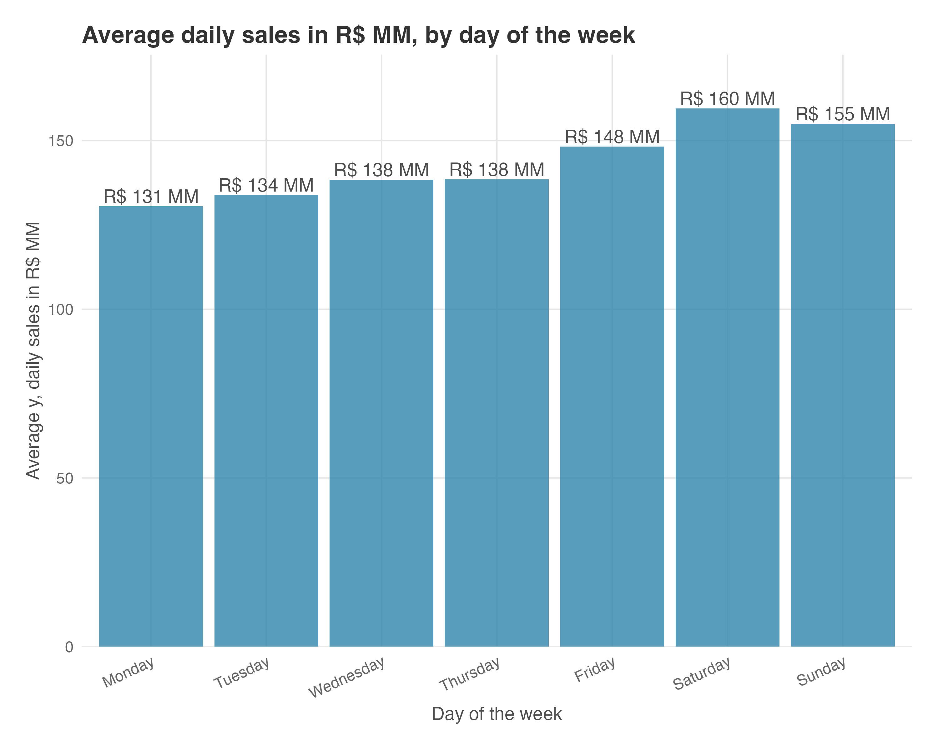
Is my series ready for ARIMA?
Before fitting an ARIMA model, you need to check whether your series is stationary — a fundamental requirement that trips up many practitioners.
What stationarity means
Imagine monitoring the temperature in a thermostat-controlled room. The reading fluctuates around 22°C — sometimes 21°C, sometimes 23°C — but it always returns to that neighborhood. That’s stationarity: the series has a stable mean, stable variance, and predictable patterns.
Now imagine the thermostat is broken and the room is slowly warming. The temperature drifts from 20°C to 25°C to 30°C. Even if the fluctuations look similar (still ±2°C), the series is non-stationary because the center keeps moving.
Why does this matter for causal inference? When we use pre-intervention data to predict a counterfactual, we’re assuming the “rules” of the series persist. If the series is non-stationary — drifting, exploding, or fundamentally changing character — those rules aren’t stable, and our counterfactual becomes unreliable.
Visual diagnostics
Plot your series and ask three questions:
Does it have a visible trend? If sales grow steadily from R$100MM to R$150MM over your pre-period, you have a trend. The series isn’t fluctuating around a constant mean.
Does the variance change? If early months show ±R$5MM swings but later months show ±R$20MM swings, the volatility is changing over time (technically called heteroskedasticity).
Are there level shifts? If the series suddenly jumps from one plateau to another (say, after a major product launch), you may have a structural break — a change in the underlying data-generating process.
If you answered “yes” to any of these, your series likely needs transformation before ARIMA can work reliably.
The Augmented Dickey-Fuller (ADF) test
The ADF test formalizes what your eyes see. It tests for a unit root — the technical term for a specific type of non-stationarity where shocks to the series persist forever rather than fading away.
Interpretation:
- p-value < 0.05: Reject the null hypothesis of a unit root. The series is stationary — good news. You can fit ARIMA with
d=0. - p-value ≥ 0.05: Cannot reject the null. The series appears non-stationary. Try differencing (see below) and re-test.
Practical workflow:
- Run ADF on your raw series. If p < 0.05, you’re done — use
d=0. - If p ≥ 0.05, difference the series once (\(Y'_t = Y_t - Y_{t-1}\)) and re-run ADF.
- If the differenced series passes (p < 0.05), use
d=1. - If it still fails, try
d=2— but this is rare. If you need more than two differences, something unusual is happening (exponential growth, structural breaks) that differencing alone won’t fix.
When and how to difference
Differencing transforms a non-stationary series into a stationary one by modeling changes rather than levels. Instead of asking “What were sales today?”, you ask “How much did sales change from yesterday?”
Decision tree:
- Linear trend (steady growth of X units/day)? → First difference (
d=1) removes it. The differenced series oscillates around zero. - Seasonal pattern (every Monday is lower, every December is higher)? → Seasonal differencing (
D=1) at the seasonal lag. For weekly data with 7-day cycles, this means \(Y'_t = Y_t - Y_{t-7}\) — comparing each Monday to the previous Monday. - Both trend and seasonality? → You may need both
d=1andD=1.
The “I” in ARIMA stands for integrated: the original series can be recovered by summing (integrating) the differenced series. An ARIMA(1,1,1) fits an ARMA(1,1) model to the first-differenced data. A technical nuance worth noting: when C-ARIMA uses differencing (\(d > 0\) or \(D > 0\)), the causal effects are initially computed in the differenced space, then “integrated back” to the original scale to produce interpretable point effects. Menchetti, Cipollini, and Mealli (2023) (Theorem 4.2) provide the distributional result for this case — the CausalArima package handles this automatically, but it’s useful to know why your confidence intervals may widen more when differencing is applied.
Warning: Differencing removes linear trends but won’t fix all problems. If your series has structural breaks (sudden level shifts from a product pivot or market shock), exponential growth, or wildly changing volatility, differencing alone isn’t enough. Consider truncating the data to exclude the unstable period, or consult a time series specialist.
Decoding ARIMA notation
When you see ARIMA(2,0,0)(2,1,0)[7], here’s what each piece means:
| Parameter | Name | Plain English |
|---|---|---|
p = 2 |
Autoregressive order | “Today depends on the last 2 days” |
d = 0 |
Differencing order | “No differencing needed — series is stationary” |
q = 0 |
Moving average order | “Don’t use past forecast errors” |
P = 2 |
Seasonal AR order | “Today depends on the same weekday from the last 2 weeks” |
D = 1 |
Seasonal differencing | “Compare each day to the same day last week” |
Q = 0 |
Seasonal MA order | “Don’t use past seasonal forecast errors” |
[7] |
Seasonal period | “Weekly cycle (7 days)” |
Reading the example: ARIMA(2,0,0)(2,1,0)[7] says: “Predict today’s value using the last 2 days, plus the same weekday from the last 2 weeks, after removing the weekly pattern through seasonal differencing.”
Common patterns:
ARIMA(1,1,0)— Each day’s change depends on yesterday’s change (integrated AR(1)).ARIMA(0,1,1)— Exponential smoothing; each day’s change depends on yesterday’s forecast error.(1,0,0)[7]— Weekly seasonality where each day depends on the same day last week.
Testing for structural breaks
A structural break occurs when the underlying relationship in your data fundamentally changes — not just a temporary shock, but a permanent shift in how the system works.
The Chow test checks whether a regression relationship changed at a specific date. It splits your data at a candidate breakpoint, fits models to each segment, and tests whether the coefficients differ significantly.
When to use it:
- Before fitting C-ARIMA or CausalImpact, run the Chow test on your pre-intervention data.
- Pick candidate dates where you suspect the world changed: major competitor entry, platform migration, pandemic onset.
- If the test detects a break within your pre-period, your counterfactual projection is built on shifting sand.
Interpreting results:
- p-value < 0.05: Evidence of a structural break at that date. The “rules” changed.
- p-value ≥ 0.05: No evidence of a break. The relationship appears stable.
Limitation: You must specify the break date in advance. The Chow test doesn’t search for unknown breakpoints. If you don’t know when the break occurred, consider the Bai-Perron test or visual inspection of the residuals for clues.
How Bayesian inference powers CausalImpact
CausalImpact uses Bayesian Structural Time Series (BSTS) models. If you’ve only worked with traditional (frequentist) statistics, the Bayesian approach can seem mysterious. Here’s the intuition.
Priors: Your starting beliefs
Before seeing any data, CausalImpact has prior beliefs about what your time series looks like. These priors encode assumptions like:
- “The trend probably doesn’t change dramatically from day to day.”
- “Seasonality effects are probably modest, not extreme.”
- “Most of your auxiliary variables probably don’t matter much.”
These aren’t arbitrary — they reflect reasonable defaults for typical business data. But they matter because with little data, the prior strongly influences results. With abundant data, the data “overwhelms” the prior and the result reflects what you actually observed.
Practical implication: If you have a short pre-period (say, 30 days), your results depend heavily on these default priors. If you have a long pre-period (200+ days), the priors become nearly irrelevant. This is one reason the “sufficient history” assumption matters — more data means less dependence on assumptions.
MCMC: Exploring the counterfactual distribution
The counterfactual isn’t a single line — it’s a distribution of possible trajectories. MCMC (Markov Chain Monte Carlo) is the computational engine that maps this distribution.
Imagine you’re trying to understand the shape of a dark cave. You can’t see the whole cave at once, so you send in a robot that wanders randomly, bouncing off walls. Over time, the robot visits every part of the cave, spending more time in spacious chambers and less in narrow passages. After thousands of steps, you can map the cave by looking at where the robot spent its time.
MCMC works similarly. It “wanders” through the space of possible parameter values, spending more time in regions that fit the data well. After thousands of iterations (the niter parameter), you can map the distribution of plausible counterfactuals. The 95% credible interval represents the range where the robot spent 95% of its time — the most plausible counterfactual values.
What niter = 5000 means: The algorithm takes 5,000 “steps” through parameter space. More iterations mean a more precise map but slower computation. The default (5,000) usually suffices. If your credible intervals seem unusually jagged or unstable, try increasing to 10,000.
Why credible intervals are more intuitive
A Bayesian credible interval directly answers the question you care about: “What’s the probability the true effect lies in this range?” When CausalImpact reports a 95% credible interval of [R$18MM, R$22MM], you can interpret this literally — there’s a 95% probability the true daily effect falls within that range.
This differs from the frequentist confidence interval, which makes a statement about the procedure (“If we repeated this infinitely, 95% of intervals would contain the true value”) rather than this specific case. For decision-making, the Bayesian interpretation is far more useful — you can directly say “we’re 95% confident the effect is at least R$18MM/day.”
Appendix 11.B: C-ARIMA with external regressors
So far, I’ve presented C-ARIMA as a univariate method — building the counterfactual entirely from the target series’ own history. But C-ARIMA also supports external regressors via the xreg parameter, just like CausalImpact uses auxiliary series. As I flagged in Rule 4, covariates are often what make the “stable patterns” assumption hold in practice — this appendix shows how to use them and when they help.
The idea is straightforward. During the pre-intervention period, C-ARIMA learns the ARIMA structure of your target series and the linear relationship between the target and your external regressors. When forecasting the counterfactual, it uses the actual post-intervention values of the regressors (which, by assumption, were unaffected by the treatment) to improve its prediction. This is the same logic CausalImpact uses — the difference is that C-ARIMA wraps it in a frequentist ARIMA framework rather than a Bayesian structural model.
When does adding X help?
Adding external regressors helps when the regressors explain variation in the target that the ARIMA structure alone cannot capture. If your target series already has clean, predictable seasonality and low noise, the ARIMA component handles most of the work and the marginal benefit of xreg is small. But if your series is noisy, or if external factors (weather, holidays, market conditions) introduce variation that isn’t purely autoregressive, the regressors can substantially reduce forecast error — and therefore produce tighter confidence intervals and a more accurate causal estimate.
In our simulation, x1 is correlated with sales but the weekly seasonality dominates the signal. So we should expect a modest improvement from adding x1 — not a dramatic one. Let’s see.
Implementation
We reuse the same data and auxiliary series x1 from Section 11.3.4.
Comparing the three approaches
The table below summarizes expected results from all three methods on the same data (true effect = R$20 MM/day):
| Method | Avg. daily effect | Uses auxiliary series? | Inference |
|---|---|---|---|
| C-ARIMA (no X) | ~R$ 18.5 MM | No | Frequentist (bootstrap) |
| C-ARIMA (with X) | ~R$ 19-20 MM | Yes | Frequentist (bootstrap) |
| CausalImpact (with X) | ~R$ 20 MM | Yes | Bayesian (MCMC) |
Several patterns emerge:
Adding
x1narrows the gap. Without regressors, C-ARIMA underestimates by ~7.5%. Withx1, the estimate moves closer to the true R$20 MM.C-ARIMA with X and CausalImpact converge. When both methods use the same auxiliary information, the difference is largely about information, not statistical machinery.
The improvement is modest here because the signal is clean. In messier real-world data — where external factors drive more of the variation — the improvement from adding regressors can be much larger.
TipRefining the decision: C-ARIMA without vs. with covariates
C-ARIMA without X: Use when you have no trustworthy auxiliary series, or when you want a conservative baseline that makes minimal assumptions. Fewer moving parts means fewer ways to go wrong.
C-ARIMA with X: Use when you have auxiliary series that are (1) correlated with your target, (2) unaffected by the intervention, and (3) you prefer frequentist inference (bootstrap confidence intervals, p-values). This gives you the information advantage of auxiliary data within a frequentist framework.
CausalImpact with X: Use when the same conditions hold but you prefer Bayesian inference (credible intervals, posterior probabilities) or want the automatic variable selection that the Bayesian state-space framework provides when you have many candidate regressors.
The real question isn’t “C-ARIMA or CausalImpact” but rather “how much auxiliary information do I want to use, and which inferential framework do I prefer?” When in doubt, run all three variants and check whether they agree.
Appendix 11.C: Why not just use REG-ARIMA?
You might be wondering: “Why all this complexity? Can’t I just fit a regression with ARIMA errors and add a dummy variable for the post-intervention period?” This traditional approach (called REG-ARIMA in the literature) is indeed widely used. But Menchetti, Cipollini, and Mealli (2023) highlight three key limitations:
No explicit causal framework: REG-ARIMA does not explicitly adopt the potential outcomes framework, making causal attribution less transparent. Because it estimates on the entire time series (before and after), the coefficient on the intervention dummy captures association without explicitly reasoning about counterfactuals.
Only level shifts: REG-ARIMA, as analyzed in Menchetti, Cipollini, and Mealli (2023), captures effects only in the form of level shifts. C-ARIMA captures any effect shape automatically because it estimates point effects at each time, not a single average. You don’t need to guess whether your effect is a level shift, a gradual ramp, or something irregular.
No temporal evolution: REG-ARIMA gives you one number (the dummy coefficient). C-ARIMA gives you a time series of effects, so you can see how the impact evolved — did it peak and fade, or build steadily?
To be fair, REG-ARIMA has a power advantage when the effect truly is a constant level shift; its simpler structure is optimized for that specific case. In Menchetti, Cipollini, and Mealli (2023)’s simulations, REG-ARIMA detected a +25% level shift with near-perfect power (1.000) while C-ARIMA reached 0.895. But that advantage comes with a trap: when the true effect is not a constant shift, REG-ARIMA can produce false positives by forcing the wrong structure onto the data. In one simulation scenario with a time-varying effect that was zero at the 3-month mark, REG-ARIMA reported power of 1.000; it “detected” an effect that didn’t exist at that horizon, while C-ARIMA correctly found no significant effect at that horizon.
As Google advises, “NotebookLM can be inaccurate; please double-check its content”. I recommend reading the chapter first, then listening to the audio to reinforce what you’ve learned.↩︎
A time series is a sequence of data points measured at successive points in time, usually at regular intervals. In digital businesses, common examples include daily sales on an e-commerce platform, hourly ride requests in a ride-hailing app, or weekly active users for a fintech product.↩︎
Use these methods when you must, but treat the results with healthy skepticism.↩︎
This “local permanence” interpretation is my pragmatic relaxation of the original assumption, which formally requires irreversibility. In practice, it works well as long as you define your analysis window to cover only the period when treatment is active. Strictly speaking, you are identifying the effect of a temporary intervention during its active window — something the original paper does not formally derive but that has become a common and well-motivated practical adaptation.↩︎
This is not a formal assumption in Menchetti, Cipollini, and Mealli (2023) but an identification implication of analyzing a single series. CausalImpact can partially relax this requirement — if the concurrent shock also affects its auxiliary series, the model can account for it. C-ARIMA with external regressors can also absorb some shared variation, though its fixed-coefficient approach is less flexible at this than CausalImpact’s state-space framework.↩︎
The Chow test is a statistical method used to check whether there is a structural break at a specific point in your time series. In practice, it splits your data into two segments (before and after a chosen date) and fits a regression model to each. If the coefficients differ significantly, the test flags a structural break, meaning the relationship in your data changed at that point. For example, in a digital business, you might use the Chow test to see if a new product launch fundamentally changed the sales trend.↩︎
Menchetti, Cipollini, and Mealli (2023) also discuss “temporal no-interference” (TSUTVA), the time-series analog of SUTVA from Chapter 6, meaning that each unit’s potential outcomes depend solely on its own treatment assignment, not on the treatment assignments of other units. However, they note that for a single treated unit (no panel dimension), this assumption is unnecessary. Since we’re analyzing one business, one platform, or one market, temporal no-interference is not a binding constraint in our setting.↩︎
To load it directly, use the example URL
https://raw.githubusercontent.com/RobsonTigre/everyday-ci/main/data/time_series_campaign.csvand replace the filenametime_series_campaign.csvwith the one you need.↩︎Figure 11.12 in the Appendix 11.A better conveys the seasonality by day of the week. There you see the higher sales on Saturdays and Sundays, and lower sales on Mondays.↩︎
A note on terminology: C-ARIMA produces frequentist confidence intervals (via bootstrap), while CausalImpact produces Bayesian credible intervals (via MCMC). They look similar visually, but their interpretation differs. A confidence interval is a statement about the procedure (“if we repeated this experiment many times, 95% of intervals would contain the true value”), while a credible interval is a statement about this specific case (“there’s a 95% probability the true effect lies in this range”). See the CausalImpact section on Bayesian inference for details. When I say “CIs” generically, I mean whichever is appropriate for the method being discussed.↩︎
Python’s auto ARIMA may select a different but equivalent specification — e.g., ARIMA(0,0,2)(1,0,2)[7] — because the search strategies and information criteria differ across implementations. Both converge on similar effect estimates, which is itself a robustness check.↩︎
But residual diagnostics and power analyses are equally important.↩︎
The R and Python p-values differ because each implementation’s auto ARIMA may select a different model specification (e.g., AR vs. MA terms), producing different residual series — both are valid diagnostic residuals for checking model adequacy.↩︎
The cost of using auxiliary series is that you need more data and you introduce new assumptions about those series (they must be unaffected by the intervention, predictive of the outcome, and stable in their relationship). When C-ARIMA is run without covariates — as we did in our example — it avoids these extra assumptions. But if you add external regressors to C-ARIMA, the same “unaffected covariates” rule applies (see Assumption 4 in Section 11.2.1).↩︎
Ideally, you want a series that predicts your outcome but remains untouched by your intervention.↩︎
An important limitation: CausalImpact assumes all covariates are contemporaneous — the model does not infer lagged relationships between series (Brodersen et al. 2015). If you believe organic search leads sales by two days, you’d need to manually shift the series before feeding it to the model. This is a modeling choice you make, not something CausalImpact discovers on its own.↩︎
By incorporating auxiliary series, CausalImpact can account for external influences that C-ARIMA would miss. But the reverse is also true: if the auxiliary series are poorly chosen or contaminated by the intervention, CausalImpact can perform worse than C-ARIMA.↩︎
This is where CausalImpact can relax C-ARIMA’s “no concurrent shocks” requirement — but only if the auxiliary series capture those shocks.↩︎
This decomposition is additive (\(y_t = \text{trend} + \text{seasonality} + \text{regression} + \text{noise}\)). If your intervention produces a multiplicative effect — say, a 15% lift regardless of the baseline level — the model is misspecified, because a 15% lift means a bigger absolute increase on high-sales days than low-sales days. The workaround: apply a log transformation to your outcome before running CausalImpact. Logarithms convert multiplication into addition (\(\log(1.15 \times y) = \log(y) + \log(1.15)\)), so the model works correctly on the log scale. Exponentiate the results to return to the original scale.↩︎
Brodersen et al.’s Figure 2 shows the full graphical model with latent state nodes. The observation equation is \(y_t = Z_t^T \alpha_t + \varepsilon_t\) and the state equation is \(\alpha_{t+1} = T_t \alpha_t + R_t \eta_t\). This state-space structure is what makes CausalImpact flexible enough to decompose your series into trend, seasonality, and regression components simultaneously.↩︎
Recall from our earlier discussion that cumulative effects are only meaningful for flow metrics like daily sales — quantities measured over an interval. For stock metrics (like total active users), summing daily values double-counts and produces nonsense; report the point effect or temporal average instead (Brodersen et al. 2015).↩︎
See the footnote in Section 11.2.3 for the distinction between confidence and credible intervals.↩︎
Recall Figure 6.11 from Chapter 6, where we saw how an overall positive correlation between two variables can reverse when we condition on a third.↩︎