13 Falsification and robustness: Stress test your results before someone else does
A/B Testing, Causal Inference, Causal Time Series Analysis, Data Science, Difference-in-Differences, Directed Acyclic Graphs, Econometrics, Impact Evaluation, Instrumental Variables, Heterogeneous Treatment Effects, Potential Outcomes, Power Analysis, Sample Size Calculation, Python and R Programming, Randomized Experiments, Regression Discontinuity, Treatment Effects
13.1 Data can debunk, but it cannot confirm
A marketplace launches a free-shipping banner. It does not show the banner to everyone. A targeting model decides who sees it, picking out the users it expects to buy. A few weeks later, the analytics team pulls the numbers: users who saw the banner generated far more 30-day profit than users who did not. The first cut puts the lift at R$7.86 per user. Someone drops it into a slide deck, the title reads “Free shipping works,” and the room is ready to keep the current targeting rule. Then someone asks whether the same number justifies exposing the whole user base.
A skeptic asks: how do you know it’s the banner, and not the kind of user the banner gets shown to? The targeting model was built to find high-intent shoppers, and those users were going to spend more anyway. The banner and the buying may be two symptoms of the same thing: a user who was already leaning toward a purchase. The R$7.86 could be mostly the banner, mostly the targeting, or anything in between. Nothing in that first cut can tell the difference.
A causal estimate is more credible when it survives tests that could expose a problem. Data can rule out implications and show that a design fails its own predictions. Even a long run of clean checks does not prove that the reported number is causal. Without those checks, the estimate is a weak basis for a budget decision.
Part II introduced methods for estimating effects: experiments, regression, instrumental variables, discontinuities, difference-in-differences, and heterogeneous effects. This chapter asks how much causal credibility those estimates deserve. Earlier chapters already used parallel trends, balance, overlap, first stages, and density checks. Here, those diagnostics become parts of one falsification workflow, applied to a single estimate before it is translated into business value (Chapter 14).
Before putting the number on trial, define what it is supposed to estimate. An estimand is the population quantity an analysis targets. The primary estimand here is the targeted-user average treatment effect on the treated (ATT): the banner’s average effect on 30-day profit among the 14,209 users who currently received it. Because the data is simulated, its truth is R$0.99. The whole-base ATE (average treatment effect) is R$0.90 across 30,000 users, while the currently untreated ATC (average treatment effect on the controls) for the 15,791 users not shown the banner is R$0.82. Those quantities are close here, but they answer different decisions. The ATT for today’s targeted users does not tell us what would happen if the banner reached today’s untreated users; a literal whole-base rollout needs evidence for that population, preferably from a randomized holdout.
Table 13.1 gives the starting estimates and primary grading target:
The raw number is precise. Precision is not the same as truth. The chapter first adds prior orders, prior profit, and pre-period sessions, which cuts R$7.86 to the intermediate R$2.19. The early placebo family diagnoses that intermediate model. We then add eligibility as an effect modifier and standardize the contrast to the currently targeted population, producing the focal observational contrast of R$1.87. Every applicable diagnostic is rerun on that focal model before sensitivity analysis bounds the remaining vulnerability. The simulated truth lets us grade full-sample targeted-user specifications against R$0.99 and keep the eligible-user truth, R$1.50, in a separate population-specific callout.
Data: All data we’ll use are available in the repository. The free-shipping dataset for this chapter is data/free_shipping_banner.csv. You can download it from the repository or load it directly by passing the raw URL to read.csv() in R or pd.read_csv() in Python.2
Packages: To run the code yourself, you’ll need a few tools. The block below loads them for you. Quick tip: you only need to install these packages once, but you must load them every time you start a new session in R or Python.
# If you haven't already, run this once to install the packages:
# install.packages(c("tidyverse", "fixest", "lmtest", "sandwich", "MatchIt", "WeightIt", "cobalt", "sensemakr", "dagitty", "specr"))

# You must run the lines below at the start of every new R session.
library(tidyverse)   # data wrangling and plots
library(fixest)      # fast regression with robust standard errors
library(lmtest)      # coefficient tests used with robust covariance matrices
library(sandwich)    # HC1 and HC3 covariance matrices for lm()
library(MatchIt)     # nearest-neighbour and other matching estimators
library(WeightIt)    # inverse-probability and balancing weights
library(cobalt)      # balance diagnostics and love plots
library(sensemakr)   # sensitivity analysis for unobserved confounding
library(dagitty)     # draw DAGs and read off testable implications
library(specr)       # specification-curve analysis in the appendix
# From the repository root, run this once to install the pinned packages:
# python -m pip install -r requirements.txt
# You must run the lines below at the start of every new Python session.
import itertools # specification-grid combinations
import pandas as pd
import numpy as np
import networkx as nx # DAG d-separation checks
import matplotlib.pyplot as plt # balance and specification-curve plots
import statsmodels.formula.api as smf # OLS with a formula interface
import statsmodels.api as sm # formula-based binomial GLM
import sensemakr # sensitivity analysis (PySensemakr)
from scipy.stats import norm, t as student_t # Fisher and Student-t intervals
from sklearn.neighbors import NearestNeighbors # nearest-neighbour matching13.2 Why causal inference is not just estimation
Suppose the team reruns the banner regression across regions, devices, and months and obtains a positive estimate each time. Those estimates are not independent confirmations if they reuse the same data and assumptions. A fake effect showing up where there should be no effect may be more informative than another favorable specification, but its weight depends on the test’s false-positive rate, its power against a plausible violation, and its dependence on the other results. A passing test supports the maintained assumptions only when it could have detected a relevant failure. It does not prove them (Eggers et al. 2024).
Karl Popper’s account of conjectures and refutations provides the practical frame (Popper 1963). You are not trying to accumulate proof that the banner works. You are trying, on purpose, to break the claim that it does, and to report whether it broke. Athey and Imbens describe placebos, validation checks, and sensitivity analyses as supplementary analyses that assess the credibility of a primary estimate (Athey and Imbens 2017). Producing an estimate is easy. The work is showing why it deserves a causal interpretation.
The same data can support more than one story. The R$7.86 lift fits a world where the banner increases spending, but it also fits one where the targeting model selects users who would have spent more anyway. Calling the analysis “data-driven” does not distinguish those stories because the observed data does not record the intent that drove targeting. To separate them, move beyond the regression output and design a check that should produce different results under the causal story and its rival.
If your explanation can absorb any outcome after the fact (lift goes up, the banner worked; lift goes down, the market was soft; lift is flat, it takes time to build habit) then it is not being tested, just narrated. State a prediction that could fail before running the check. If the adjusted treated-control comparison is valid, the banner should be associated with neither an outcome it cannot affect nor meaningful differences in relevant pre-treatment variables. Stake out the prediction before you look, and a failed check means something.
The most useful check is the one aimed at the design’s weakest assumption, because it has a real chance to overturn the result. A check the design passes no matter what tells you nothing. Decide what result would convince you that the causal claim is wrong, then look for it.
Pre-trends, placebo tests, balance checks, first-stage diagnostics, and density checks at a cutoff all try to make a design fail where a sound design should hold. You have used falsification tests throughout the book under other names. This chapter names them, connects them, and adds tools for stress-testing one headline estimate.
Key takeaway. Estimation gives you a number; identification gives you the reason to read that number as causal. The chapters before this one taught you to produce the number. This one is about whether you have earned the right to call it an effect, and the way you earn it is by trying, in good faith, to break it.
13.3 What falsification actually is
Direct placebo tests follow the same three-step recipe (Eggers et al. 2024): name the assumption, build a check whose true effect is zero under the maintained assumptions, and preserve the parts of the main analysis that carry the problem being tested. The chapter also uses related diagnostics—balance, overlap, first stages, and d-separation—that test observable implications without following that exact zero-effect template.
First, name the assumption each check targets and state what its failure would affect. Some failures bias the estimate. The intermediate banner regression, for example, assumes that treated and untreated users are comparable after adjustment; otherwise R$2.19 is not the banner effect. Other failures leave the point estimate unchanged but invalidate its uncertainty. Users in the same group may share unmodeled behavior, making the confidence interval too narrow. The remedies differ: better standard errors do not correct confounding, and adding a control does not fix dependent errors. State the failure before designing the check so that a pass has a defined meaning.
The second step is to build a check where the true effect is zero by construction. Alter one of three things—the outcome, treatment, or population—so that the rebuilt quantity must be null if the maintained design and measurement assumptions hold. Call this the no-effect-by-construction condition: you are not merely hoping the answer is zero; you have stated an implication that can fail. Change the outcome to something the banner cannot plausibly move, like profit in a product category free shipping does not apply to. Change the treatment to a fake exposure with no causal path to profit. Change the population to users for whom the treatment is inert, shoppers who were shown the banner but cannot redeem free shipping at all. A non-zero result is evidence against the maintained implication, but the source may be confounding, functional form, measurement, or another assumption the check relies on. Eggers, Tuñón, and Dafoe call this the No Average Treatment Effect, or NATE, assumption (Eggers et al. 2024). Here, we keep the plainer phrase no effect by construction.
Third, preserve the parts of the main analysis that transmit the problem the placebo is meant to detect. Reuse the estimator, controls, and uncertainty procedure when that keeps the main and placebo assumptions aligned. Make any change required for a valid placebo, such as conditioning on the real treatment in a placebo-exposure test. The analyses need not be mechanically identical. The placebo is informative when its effect is plausibly zero, it behaves as expected when the main assumptions hold, and it reproduces the relevant bias or inference failure when they do not (Eggers et al. 2024).
Before calling a null reassuring, judge power against a pre-specified materiality threshold. Before looking at a regression placebo, state the largest false effect that would leave the business decision unchanged, in outcome units. Call it a pass only if its interval lies within that band; merely including zero is not enough. If no defensible band exists, report the estimate and interval without calling the check resolved. Balance, overlap, effective sample size, robustness ranges, and Monte Carlo calibration use their appropriate descriptive summaries rather than this interval rule.
That brings us to the line this chapter repeats until it is reflex: a failing falsification test is evidence against a maintained implication; a passing one is limited reassurance, never proof. The two directions are not symmetric. When a valid, well-powered placebo that should be zero comes back clearly non-zero, the design has failed that implication. When it comes back null, you have only failed to catch a problem at that spot, with that much power. Other flaws can still hide elsewhere. The right reading is probabilistic: a null placebo shifts your belief toward the maintained design, but does not settle the question (Eggers et al. 2024). The checks in one analysis are often correlated, so their agreement should not be sold as independent corroboration.
You have used this logic throughout the book. Checking parallel trends is a placebo on the pre-period, the no-effect-by-construction condition applied to time (Chapter 9, Section 9.5.5). A balance table asks whether pre-treatment characteristics differ enough to threaten comparability (Table 3.1, Section 4.2.5). Live experiments have their own checks: sample-ratio mismatch asks whether users split as assigned, while Twyman’s Law tells you to investigate results that look unusually different before believing them (Section 4.2.6). A first stage is the mirror-image check for an instrument, the place an IV is supposed to move, where a null would sink relevance. A pre-period outcome placebo for an instrument instead probes independence or exogeneity: an association before treatment suggests that the instrument and outcome share prior causes. It does not test the exclusion restriction, which is not directly testable in a just-identified IV model (Section 7.4). The next section applies the same logic to the banner data.
13.4 The falsification tests you already run
Each subsection applies a diagnostic to the banner data and points back to the earlier design where it first appeared. The direct placebos change the outcome, treatment, or population so that the maintained assumptions imply a value near zero. Balance, overlap, and d-separation test other observable implications rather than substituting a fake outcome, treatment, or population. Because the data is simulated, the known DGP helps identify why an implication fails.
The initial checks use the intermediate core-controls model. The robustness section later defines the focal eligibility-interaction model and collects the applicable focal rechecks in one table.
Every regression-based check reports an estimate and interval. A nonzero placebo contradicts its maintained implication; a near-zero result provides limited reassurance only when the test could have detected a material problem.
13.4.1 Placebo in time: a “fake effect” before the banner existed
Event-study leads are placebo estimates. Under no anticipation and the design’s pre-period trend restrictions, their population values should be zero. A nonzero lead shows that the design or specification conflicts with those restrictions. Possible explanations include differential pre-trends, anticipation, time-varying confounding, functional-form misspecification, contamination from heterogeneous post-treatment effects in a conventional staggered-TWFE event study, and Ashenfelter’s dip when treatment follows a temporary pre-treatment outcome decline. The lead coefficients alone do not identify which explanation applies (Section 9.5.3.2, Section 9.5.5).
The same logic appears in two earlier checks: a fake intervention date in time-series analysis (Section 11.2.4, Section 11.3.5.1) and an A/A test before an experiment (Section 4.2.5). Roth’s point is narrower than “clean leads prove parallel trends”: pre-period coefficients test an implication related to parallel trends, often with low power, and conditioning on passing that test distorts later inference (Roth et al. 2023). The TWFE chapter uses a joint F/Wald test of all pre-treatment coefficients; Section 9.5.3.2 provides the R and Python implementation.
The banner version is the simplest case of the recipe. The banner launched on a specific day; it cannot have changed anything that happened before that day. So take the pre-treatment outcome, profit_pre, each user’s profit in the window before the banner existed (a separate measure from the prior_profit control), and run the intermediate core-controls specification, swapping only the outcome. If the maintained comparison is clean, the adjusted treated-control gap on profit_pre should be about zero because a future banner cannot reach into the past.
It is not zero. The intermediate placebo-in-time contrast is R$1.59 [R$1.32, R$1.86]. Treated users were already more profitable than controls before the banner appeared. That pattern is evidence against the intermediate model’s clean-comparison implication and is consistent with the targeting model selecting users who were already more profitable. Figure 13.1 also shows the focal recheck introduced later; it remains R$1.60 [R$1.33, R$1.88].
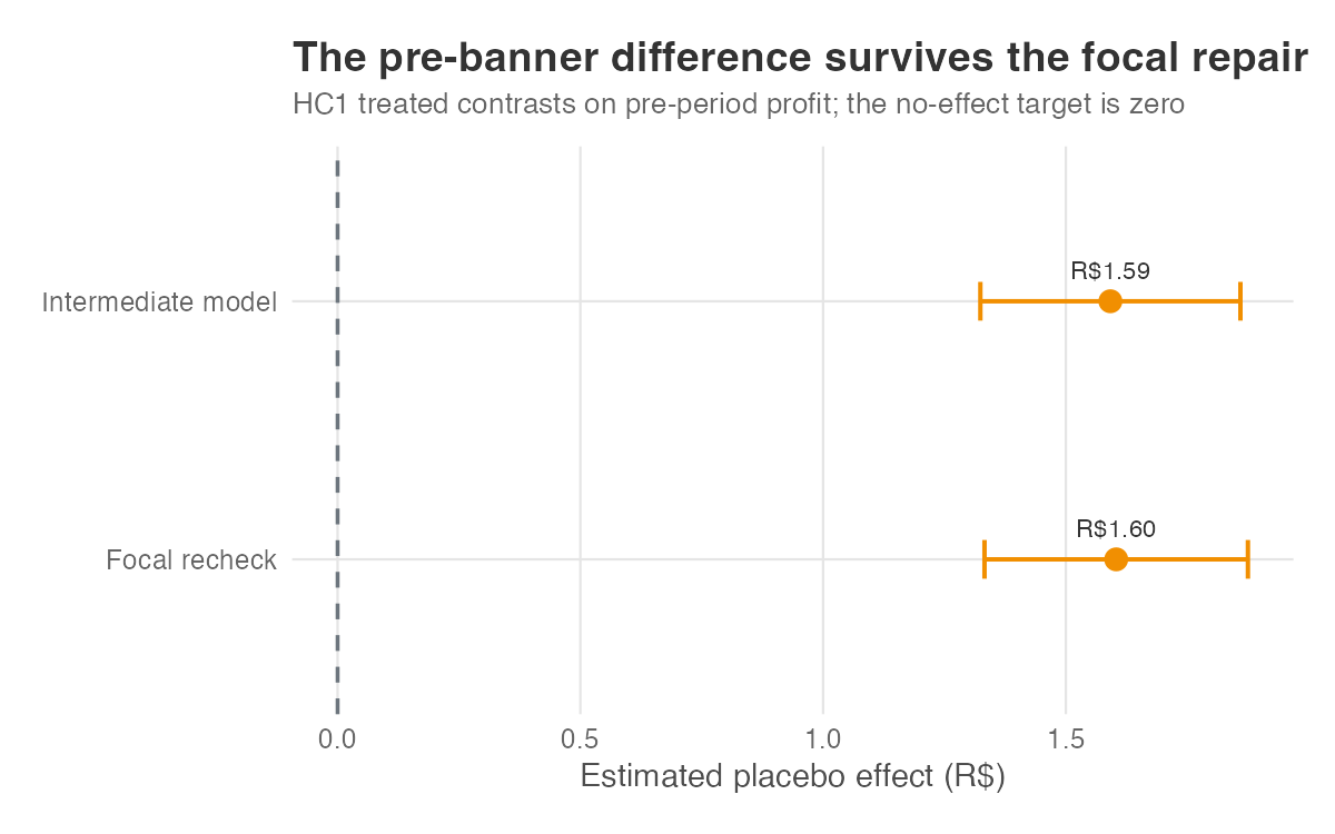
Interpret the nonzero placebo. A non-zero placebo-in-time effect does not show that the banner has no effect. It shows that treated and control users already differed before treatment, so the post-treatment gap begins from an unequal baseline. Conditioning on the pre-treatment behavior used by the targeting model is the same adjustment that shrank the naive estimate. Because the placebo remains nonzero after that adjustment, the controls did not fully close the pre-treatment gap.
13.4.2 Negative-control outcomes: an effect where the banner cannot reach
You have run this check before as covariate balance in regression discontinuity. There, you applied the RDD to a variable the cutoff should not move (age, when the threshold concerns something else) and treated a jump as a warning rather than a finding (Section 8.2.1, Figure 8.4). RDD adds another falsification in the density-at-the-cutoff test, which looks for bunching that suggests units manipulated which side of the threshold they reached (Figure 8.5). Time-series analysis uses the same logic: a control or auxiliary series used for prediction must be unaffected by the intervention, or the comparison becomes circular (Section 11.3.1). Each check points the estimator at a quantity whose true effect is zero by definition.
The logic generalizes into the idea of a negative-control outcome (also called a null outcome) (Lipsitch et al. 2010). Choose an outcome that shares the confounding path with the focal outcome but not the causal path. Here the confounding path is shopping intent: the same hidden eagerness that made the targeting model show someone the banner also makes them spend more across the board. So pick an outcome that intent drives but the banner cannot: noneligible_category_profit, spend in product categories the free-shipping offer does not even apply to. In this simulation, the DGP gives the banner no causal path to this outcome. If selection were absent, the adjusted association would be zero.
In an applied analysis, this is a valid negative-control outcome only if the offer cannot change noneligible-category profit directly or indirectly. Basket substitution, complementary purchases, a shared checkout threshold, or reallocating a fixed shopping budget can create a causal path from the banner to this outcome. Document why those paths are absent; otherwise a nonzero result may reflect a real treatment pathway rather than confounding.
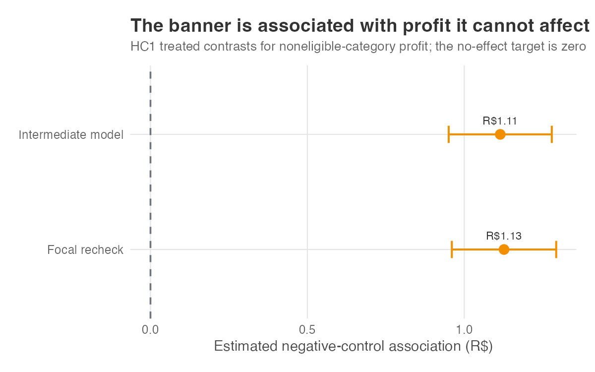
It is not zero. The intermediate association with the negative-control outcome is R$1.11 [R$0.95, R$1.28]. That is evidence against the claim that the core controls make treated and untreated users comparable. Residual selection is a plausible explanation, but the diagnostic alone does not identify its source. As Figure 13.2 shows, the focal recheck later is nearly unchanged at R$1.13 [R$0.96, R$1.29].
A balance table applies the same zero-target logic to a pre-treatment covariate rather than an outcome. Random assignment makes treatment independent of baseline characteristics in the assignment distribution, but chance imbalances can appear in a realized sample. In observational data, large or systematic gaps warn that the groups differ on measured covariates. Balance on measured covariates does not establish unconfoundedness. The overlap-and-balance section later applies this logic to the banner covariates (Section 13.4.5).
A real effect tends to be specific: concentrated where the mechanism acts and absent where it does not. Free shipping should move spend in eligible categories and leave ineligible ones flat; an association that also appears where the mechanism cannot reach is consistent with a shared cause or another failure of the maintained model (Lipsitch et al. 2010). We return to this specificity pattern later in the chapter when we read the family of checks together.
Key takeaway. A negative-control outcome shares plausible causes with the focal outcome but has no causal path from the treatment. On the intermediate banner model, both the placebo in time (R$1.59 [R$1.32, R$1.86]) and the negative-control outcome (R$1.11 [R$0.95, R$1.28]) violate their zero implications. They are related diagnostics from one observational design, not independent confirmations.
13.4.3 Placebo treatments: an effect from an assignment that did nothing
You have done a version of this in the heterogeneous-effects chapter, where permuted treatment labels form a null reference distribution (Section 12.7). Here we need to separate that null calibration from a negative-control exposure. A random permutation deliberately destroys the targeting structure; it checks whether the estimation procedure returns a null for a deterministic irrelevant label. A negative-control exposure should preserve a cause of real assignment while having no causal path to the outcome (Lipsitch et al. 2010).
The code builds both. The null permutation shuffles the treatment labels by a fixed rule rather than a random draw, so R and Python assign identical placebo labels and report the same number. The score-preserving fake exposure instead takes the untreated users the targeting model rated highest and labels them as if they had been exposed. It labels 7,479 of them, the count that gives the fake exposure the same share of the untreated pool that real exposure has of the whole base: floor(14,209 / 30,000 × 15,791). They never saw the banner, but the fake label carries the same selection pressure the real one does. Both regressions keep the real treated variable in the model; otherwise the fake label could stand in for actual exposure instead of testing what is left after it.
The two checks answer different questions. The deterministic permutation returns R$-0.06 [R$-0.30, R$0.17] for one fixed irrelevant label. Because no materiality band was pre-specified, report the estimate and interval rather than calling this a passed placebo. It also does not calibrate the estimator’s null distribution or rejection rate; that requires repeated assignments, as in the placebo-unit exercise below. The score-preserving fake exposure returns R$1.59 [R$1.23, R$1.95]. This shows that score-based selection still predicts profit after holding the real treatment and core controls fixed. With the focal interaction, the estimates become R$-0.05 [R$-0.28, R$0.18] and R$1.38 [R$1.02, R$1.73]. The focal model reduces the score-based warning but does not remove it.
Condition on the real treatment. A fake exposure fitted on its own can inherit the real exposure’s association with profit. Keeping treated in the model makes the placebo coefficient describe what the fake label adds after actual banner exposure is held fixed.
13.4.5 Balance and overlap: are we comparing comparable users?
Balance and overlap answer different questions. A balance table compares pre-treatment covariates between treated and untreated groups (Table 3.1, Section 3.4.3). Under a specified assignment design, those covariates have a placebo-like zero implication. Overlap or positivity asks whether each type of user in the target population appears in both treatment groups so that a comparison is possible (Chapter 6). It is a support condition, not a placebo test.
For balance, the zero target is straightforward. A pre-treatment covariate is fixed before the banner exists, so the banner cannot move it. Standardized mean differences (SMDs) put covariate gaps on a common scale; a love plot shows those gaps before and after adjustment. We use the common \(|\text{SMD}| < 0.10\) threshold as a descriptive screen, not as one hypothesis test per covariate. Propensity-score overlap compares the estimated probability of treatment across groups and exposes regions where one group has no credible counterpart. Propensity weighting turns those probabilities into weights for a target-population comparison (Hirano and Imbens 2001). Propensity-score matching works in two stages: it first estimates each user’s probability of treatment from observed pre-treatment covariates, then matches treated and untreated users with similar scores.3
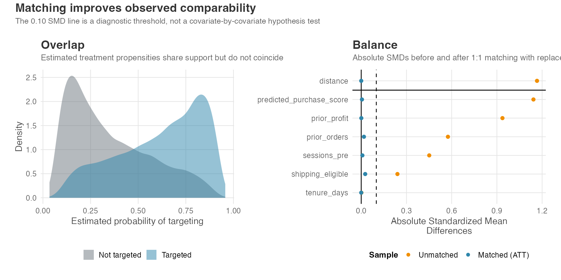
On the banner data, Figure 13.3 shows that the propensity distributions overlap but do not coincide. Matching uses all 14,209 treated users but only 6,017 distinct control users, because matching with replacement lets one control stand in for several treated users. Counting those repeats gives the matched controls an effective sample size (ESS) of 2,727 equally weighted controls. The largest absolute ATT-standardized SMD is 0.026, well below the 0.10 diagnostic threshold. That is good observed balance, not evidence that latent intent is balanced.
First, good observed balance is necessary but not sufficient. The latent shopping intent that no column captures can still differ after every SMD clears the threshold. Second, an SMD table is a threshold diagnostic, not a batch of null-hypothesis tests. If you need a formal claim that differences are negligibly small, pre-specify equivalence margins and treat those tests as a correlated family (Hartman and Hidalgo 2018). Do not retrofit one p-value per covariate onto a love plot.
Key takeaway. Matching brings the largest observed SMD down to 0.026, using 6,017 unique controls with control ESS about 2,727. Those are strong descriptive balance diagnostics. They do not address the unobserved intent that drives both targeting and profit.
13.4.6 d-separation: testing a DAG’s observable implications
The causal-assumptions chapter left this test open (Section 6.4.2). d-separation is the graphical rule for deciding whether a conditioning set blocks every path connecting two variables in a DAG. When all paths are blocked, the graph implies a conditional independence that can sometimes be checked in observed data. If the data contradicts that prediction, the result is evidence against that implication, not a verdict on the whole causal story.
Here the test targets a zero conditional correlation. If the candidate graph is right, two variables must be unrelated once the right set of others is held fixed. We check that by regressing each of the two on that set and correlating what is left over, which assumes those relationships are linear. That puts the graph and the method on trial together: a leftover correlation that is not zero tells you something in the pair is wrong, not which one. A missing arrow and a curved relationship the straight-line fit could not absorb look the same here.
The candidate graph says that pre-treatment behavior drives both the score and profit, the score drives exposure, and exposure drives profit. It omits shipping eligibility and latent shopping intent. The graph implies three marginal independencies among prior_orders, prior_profit, and sessions_pre, plus score-profit independence after conditioning on exposure and the core controls. We report all four, using the adjusted score-profit correlation as the primary test because it is closest to the identification question. Figure 13.4 keeps the candidate graph visible beside the DGP-consistent correction.
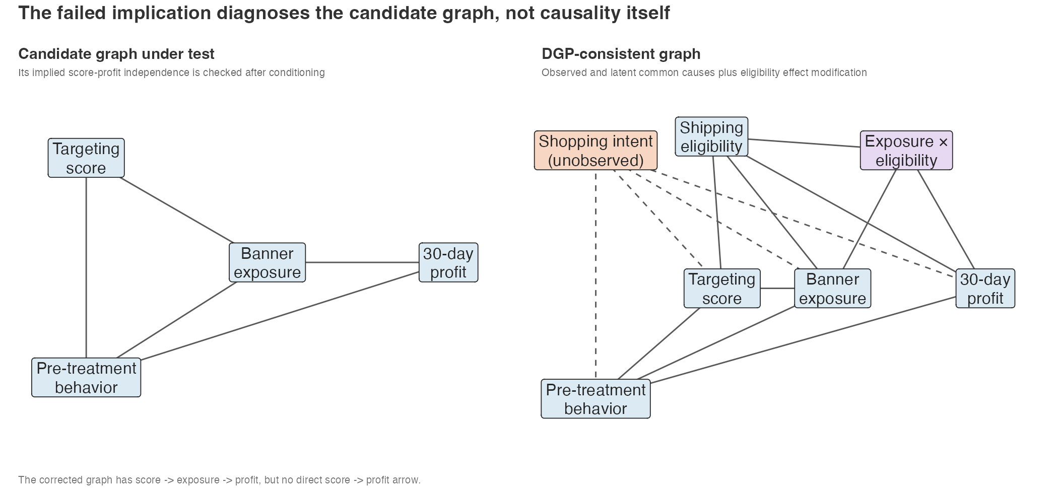
prior_orders, prior_profit, and sessions_pre into one pre-treatment behavior node so the figure stays readable; the code keeps the three variables separate, which is what makes the three marginal independencies testable.
All four candidate implications fail. The three marginal correlations are 0.73 for orders-profit, 0.22 for orders-sessions, and 0.37 for profit-sessions, none of them close to the zero the graph claims. The primary adjusted score-profit correlation is 0.12 [0.11, 0.13]. After the focal eligibility interaction is added, that last correlation falls to 0.11 [0.09, 0.12] but remains away from zero.
In the known DGP, score and profit are associated through shared observed and latent causes and through score -> treated -> profit; there is no direct score-to-profit arrow. After focal conditioning, the remaining correlation is consistent with the omitted latent intent path. The tests alone do not identify that omitted cause: missing eligibility structure, functional form, and measurement are alternative explanations in a real application.
The conclusion is implication-specific. The candidate graph and linear conditioning model do not reproduce the claimed independence. The corrected graph explains why that implication need not hold in this simulation, while the statistical check alone would not tell us which correction is right.
13.4.7 Two habits that keep placebo tests honest
Define the placebo family before looking at the results. The banner checks reuse the same users, covariates, and outcomes, so they are correlated; neither the independence formula nor the story that each result is a fresh confirmation applies. Read their estimates, intervals, and maintained implications together. If the analysis makes a formal family of inferential claims, use a joint or multiplicity-aware procedure appropriate to that pre-specified family (Section 5.5.2). The event-study leads discussed earlier form one coherent family: one model, one set of coefficients, one joint null (Section 9.5.3.2). The checks in this section do not. They fit separate models to overlapping users, so no correction makes them independent evidence or removes the bias they share. The balance SMDs remain threshold diagnostics and are not folded into that family as one hypothesis test per covariate.
The second habit is to decide in advance what will count as evidence. If you choose which placebo matters after seeing the results, you can always protect your claim: ignore the checks that detect an effect and highlight those that do not. Write down the tests, outcomes, and pass/fail thresholds before you look at the data, just as you would define the causal question in advance (Section 3.1). Pre-registration records those choices. A passing result carries weight only when the same test could also have counted against your claim.
These habits are part of the design, not a footnote after the results. A pre-specified check can come out against the claim; an improvised check can always be reinterpreted. Report which implication failed, what uncertainty surrounds the estimate, how the checks relate to one another, and what alternative explanations remain.
Falsification checks ask where the effect should be zero. Robustness checks ask whether the estimated effect survives other defensible choices about controls, estimators, and samples. Stability across those choices increases confidence that the estimate is not an artifact of one analytic decision.
13.5 Robustness and specification tests
Every analysis involves choices about controls, estimators, and samples. More than one choice may be defensible, so a colleague rebuilding the analysis could reasonably take another path. A robustness test asks whether the conclusion changes under those alternatives. When the headline number barely moves across a grid of defensible choices, you have evidence that it is not an artifact of one particular path through the observed data; whether it is causal still depends on the identifying assumptions shared by the grid.
Read that grid for effect-size stability, not statistical significance. A row of stars across six specifications mostly tells you the sample is large, not that the effect is stable. The question for a decision is whether the magnitude stays in a band tight enough to support the same action across defensible choices. A large swing can matter even when every row is statistically different from zero.
Use this template for every robustness move (Huntington-Klein 2021):
- Name the baseline assumption.
- Predict the direction of bias if it fails.
- Give a dataset-specific reason it may fail.
- State the alternative specification.
- Before running it, decide what movement would mean.
A check you cannot interpret in advance is a number you can rationalize after the fact.
Take the banner’s core specification through that template once. The baseline assumes the pre-treatment behavior we control for (orders, profit, sessions) captures the selection the targeting model acted on. If it does not, the bias points up, because the model favored high-intent users who spend more for reasons we have not fully measured. We suspect it here because the placebo-in-time and negative-control checks already fired: the controls helped but did not fully close the gap. The real targeting score can help because it proxies the latent intent that ordinary controls miss. A large change after adding it shows that the estimate depends on this targeting-process lever; movement alone neither proves bias nor identifies its direction. In another setting, adding a variable that predicts treatment but not the outcome can amplify residual confounding rather than reduce it (Cinelli, Forney, et al. 2024).
Purpose separates robustness checks from specification fishing. Each specification in your grid should answer a specific threat you can name, not exist because the software made it easy to run (Neumayer and Plümper 2017). Choosing one preferred estimate from forty regressions is specification fishing. A six-row grid is useful only when each row addresses a documented weakness and its interpretation was set in advance. The difference is not the number of specs but whether you can say, for each one, which assumption it stresses and what its result would mean. A grid assembled this way is interpretable; a grid assembled by clicking through options is just a wider net for false positives.
13.5.1 Align the focal model with the targeted-user ATT
The intermediate core model assumes one constant treatment effect even though eligibility determines whether free shipping can matter. The focal model adds an interaction between treatment and eligibility, and centers eligibility at its observed share among treated users, 0.659 (65.9% of them are eligible):
\[ \begin{aligned} \text{eligibility\_centered}_i &= \text{shipping\_eligible}_i \\[0.35em] &\quad - \widehat{\mathbb E}[\text{shipping\_eligible}_i \mid \text{treated}_i = 1]. \end{aligned} \]
That centered variable enters the focal specification:
\[ \begin{aligned} \text{profit\_30d}_i =\ & \beta_0 + \beta_1\,\text{treated}_i + \beta_2\,\text{eligibility\_centered}_i \\[0.35em] & + \beta_3\,\bigl(\text{treated}_i \times \text{eligibility\_centered}_i\bigr) \\[0.35em] & + \beta_4\,\text{prior\_orders}_i + \beta_5\,\text{prior\_profit}_i + \beta_6\,\text{sessions\_pre}_i + \varepsilon_i \end{aligned} \tag{13.1}\]
With this centering, \(\beta_1\) is the focal observational contrast standardized to the currently targeted population. It is R$1.87 [R$1.60, R$2.13] with HC1. That interpretation depends on the treatment-effect function being represented by the treatment-by-eligibility interaction. If the score, prior behavior, region, device, or another covariate modifies the effect, the model must include those interactions. Centering averages the fitted contrast over the treated eligibility mix; it does not standardize unmodeled heterogeneity or identify the ATT.
Without centering, the same fitted model gives R$1.25 for ineligible users, R$2.18 for eligible users, and R$0.94 for the gap between them. Both parameterizations predict identical profit for every user; only the coefficient’s interpretation changes. Adding the interaction changes the specification. Neither the interaction nor the centering establishes causal identification.
That interval treats the centering constant as known, so it omits uncertainty from estimating it.
Every applicable diagnostic is then rerun on the focal model. The changes are modest, so the synthesis from this point onward uses the focal column rather than the earlier intermediate values.
| Diagnostic | Intermediate core model | Focal recheck |
|---|---|---|
| Placebo in time | R$1.59 [R$1.32, R$1.86] | R$1.60 [R$1.33, R$1.88] |
| Negative-control outcome | R$1.11 [R$0.95, R$1.28] | R$1.13 [R$0.96, R$1.29] |
| Deterministic null permutation | R$-0.06 [R$-0.30, R$0.17] | R$-0.05 [R$-0.28, R$0.18] |
| Score-preserving fake exposure | R$1.59 [R$1.23, R$1.95] | R$1.38 [R$1.02, R$1.73] |
| Ineligible placebo-unit contrast | R$1.12 [R$0.70, R$1.54] | R$1.25 [R$0.86, R$1.64] |
| Residual score/outcome correlation | 0.1188 [0.1076, 0.1300] | 0.1058 [0.0946, 0.1170] |
The placebo-treatment rows add the placebo indicator as one more regressor on the right-hand side of Equation 13.1. The placebo-in-time and negative-control rows keep Equation 13.1 unchanged and swap only the outcome. The residual score/outcome row residualizes both variables on the focal right-hand side rather than the intermediate one. The ineligible placebo-unit row is the one exception: it is the treated coefficient of the same fitted model written with raw shipping_eligible in place of the centered version, which reads the contrast at eligibility zero instead of at the treated eligibility mix.
13.5.2 Check the focal model across defensible choices
Figure 13.5 compares six defensible analytic choices while keeping the focal interaction fixed: core controls, context covariates, the targeting score, common-support trimming, ATT weighting, and 1:1 nearest-neighbor matching with replacement. The rows form two clusters. Core controls, context controls, and common-support trimming remain near R$1.865. Score-informed adjustment, IPW, and matching fall between R$1.08 and R$1.22. The targeting-process lever moves the estimate. The raw R$7.86 comparison stays outside the six adjusted specifications as a baseline.
Every row uses the full-sample treated eligibility share as its centering constant, so each coefficient is standardized to the same focal population. The estimation samples and weights still differ. Common-support trimming drops 18 users, including 10 treated users; the targeted-user truth in that trimmed sample is essentially unchanged at R$0.99 after rounding. IPW changes the weights, and matching replaces the full control sample with reused nearest neighbors.
Common-support trimming here keeps observations inside the overlap of the observed targeting-score ranges. Shared minima and maxima do not establish practical positivity; one group may still be sparse within that range. Before calling support adequate, show the score or propensity density by treatment group, the largest weights, and ESS.
Read the IPW estimate of R$1.22 [R$0.88, R$1.56] only as sensitivity to observed-targeting adjustment. It is closer to the simulated truth but still 23% high, and its two tested headline placebos still fire. The IPW placebo-in-time estimate is R$0.63 [R$0.29, R$0.97]. The IPW noneligible-category placebo estimate is R$0.39 [R$0.18, R$0.60]. No other IPW placebo is tested here, and this row is not a preferred causal estimate.
The reported IPW interval conditions on the estimated weights: HC1 from the weighted regression does not include uncertainty from fitting the propensity model. Before using this row for inference, report the treated and control weight distributions and ESS, check practical positivity, and use a variance estimator or bootstrap that accounts for estimated weights. Apply the same rule in R and Python.
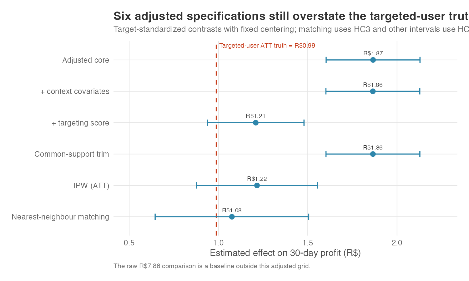
Report each grid row rather than averaging them. The R$1.08–R$1.87 range is substantive: the estimates fall when the analysis uses the targeting process more directly. The matching coefficient is R$1.08, with a conditional interval of [R$0.65, R$1.51] computed with HC3 standard errors. Treat that interval as descriptive. HC3 from the weighted outcome regression is not a matching-specific variance estimator and does not account for estimating the propensity score or selecting and reusing controls. For inference, use matching-aware uncertainty estimation and report match-distance and reuse diagnostics.
A robust-but-biased estimate is still biased. These specifications vary observed-data choices but share the latent-intent threat. Every point estimate remains above the targeted-user truth R$0.99. Their agreement says the result is not driven by one observed-data choice; it does not remove the shared bias.
Changing the population changes the question. Restricting the core model to shipping-eligible users produces R$2.27 [R$1.93, R$2.60]. Its grading target is the eligible-targeted ATT, R$1.50, not the R$0.99 truth for all targeted users. This eligible-only result is not part of the six-specification same-population grid.
Consensus is not correctness. When every specification leans on the same identifying assumption (here, that the observed covariates capture selection) they can agree while sharing the same bias. A stable grid rules out spec-dependence; it does not rule out shared bias. The sensitivity analysis ahead quantifies how strong an omitted confounder would have to be, while a randomized design would change the assignment mechanism that creates the shared threat.
Robustness checks are method-specific. In regression discontinuity, report the effect across defensible bandwidths and kernels (Section 8.2.3, Table 8.1). In difference-in-differences, a heterogeneity-robust estimator addresses staggered timing, but it does not repair violations of parallel trends (Section 10.6). Treat those as separate threats: compare estimators for treatment-effect heterogeneity, then use a sensitivity analysis that bounds how far post-treatment trends may depart from the pre-period pattern (Rambachan and Roth 2023).
When the grid grows large, a specification curve plots the estimate across every pre-declared combination of analytic choices (Simonsohn et al. 2020). Multiverse analysis extends the same idea through the full cleaning and coding pipeline (Steegen et al. 2016). Both generalize this six-row grid; the appendix gives a starting point.
Key takeaway. The six same-population focal specifications range from R$1.08 to R$1.87, above the targeted-user truth R$0.99 and far below the raw R$7.86. The grid describes sensitivity to observed-data choices. It cannot clear the latent-intent threat shared by every row.
13.6 Sensitivity to unobserved confounding
Each check so far has tested an observable implication. In the focal recheck, the placebo in time is R$1.60 [R$1.33, R$1.88], the negative-control outcome is R$1.13 [R$0.96, R$1.29], and the score-preserving fake exposure is R$1.38 [R$1.02, R$1.73]. But the focal model still rests on the assumption that observed controls capture the selection the targeting system acted on. A truly unobserved confounder cannot be inspected directly.
So the question changes from whether hidden confounding is absent to how strong it would have to be to overturn the focal result. Sensitivity analysis does not remove bias. It translates an unobserved-confounding concern into a calibrated threshold that can be compared with observed covariates (Cinelli and Hazlett 2020).
The partial-\(R^2\) sensitivity framework parameterizes omitted-variable bias with two quantities: the residual association of a hypothetical confounder with treatment and with the outcome. We apply it to \(\beta_1\) from Equation 13.1, estimated by ordinary least squares with classical standard errors — the homoskedastic ones, not the HC1 robust standard errors the chapter reports for the focal contrast and its diagnostics.4
The Robustness Value (RV) summarizes this sensitivity. At q = 1, the focal RV is 0.077: unobserved confounding with balanced strength of about 7.7% in both residual treatment and residual outcome associations could reduce the classical focal estimate to zero. The RV at \(\alpha = 0.05\) is 0.067, the corresponding threshold for moving the estimate past statistical significance. Their closeness reflects the precise classical estimate; fragility is judged from the levels and substantive benchmarks, not from the gap between the two RVs.
The treatment’s partial \(R^2\) with the outcome is 0.0065. This is the share of residual outcome variation associated with the focal treatment contrast once the model’s other terms are accounted for. It describes the coefficient’s footprint; it is not, by itself, a causal-strength measure. The same calculation also reports an extreme scenario: a confounder that explained all residual outcome variation would need to explain only 0.65% of residual treatment variation to account for the estimate. That is a low threshold, not reassurance.
Use prior_profit to interpret the sensitivity thresholds. An omitted confounder with the same residual associations as prior_profit would have a partial \(R^2\) of 0.0946 with treatment and 0.1666 with the outcome. The formal 1× bound aligns those associations in the direction that most reduces the banner coefficient. The adjusted coefficient is R$-1.19. This is a worst-case sensitivity bound, not a predicted corrected effect.
prior_profit is a calibration benchmark, not evidence that an omitted confounder with those exact relationships exists. In this simulation we know that latent shopping_intent is present because we know the DGP. Real analysts do not know the ground truth, so they cannot run the check below in an applied analysis.
The simulation lets us run one explicitly oracle-adjusted audit. Adding the actual latent intent variable to the focal regression gives a treated coefficient of R$0.91 [R$0.64, R$1.17]. The confounder’s raw partial \(R^2\) is 0.041 with treatment and 0.040 with the outcome. This coefficient is not the truth itself: the targeted-user ATT truth is a DGP average, while R$0.91 is a regression coefficient adjusted with information an analyst would not observe. It is also not the formal 1× bound, which asks a worst-case calibration question.
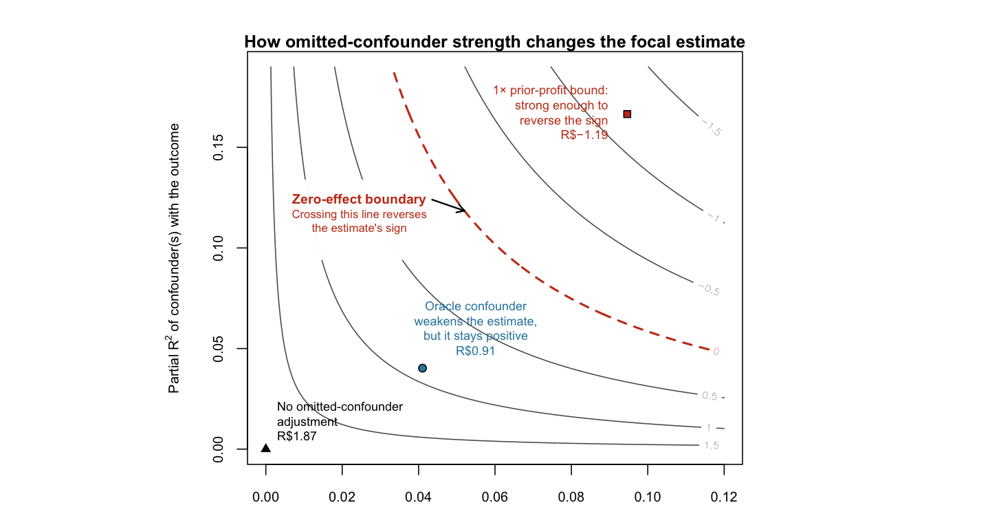
In Figure 13.6, the horizontal axis is a hypothetical confounder’s residual association with treatment and the vertical axis is its residual association with the outcome. Each contour shows the focal treated coefficient after adjustment; the red zero contour marks where the coefficient changes sign. The oracle-confounder point uses its raw partial-\(R^2\) coordinates and reproduces the fitted R$0.91 coefficient. The formal 1× prior_profit point lies beyond the zero contour and gives the R$-1.19 adverse-corner calibration. The two markers share the same axes but represent different calculations.
The reported sensitivity calculation uses the classical OLS fit so that its RVs and partial-\(R^2\) quantities match the chapter’s numerical contract. The focal HC1 interval and this classical-OLS sensitivity calculation therefore answer related but distinct questions.
The partial-\(R^2\) bound is one entry in a small family of formal sensitivity tools, each suited to a different setting. We introduce three alternatives here; the appendix develops the Masten–Poirier breakdown point. Oster’s \(\delta\) asks how strong selection on unobservables would have to be relative to selection on the observables you already control for, reading coefficient and \(R^2\) movement as you add controls (Oster 2019). The E-value translates the same worry onto the risk-ratio scale common in epidemiology, reporting the minimum confounder–exposure and confounder–outcome association needed to explain away an effect (VanderWeele and Ding 2017). The Masten–Poirier breakdown point drops the linear-model scaffolding entirely and asks, nonparametrically, how much the as-good-as-random assumption can be relaxed before the conclusion no longer holds (Masten and Poirier 2018, 2020), with nonparametric estimation and inference developed in Masten et al. (2024). Each parameterization asks how robust the result is to an assumption that cannot be tested directly.
There is no universal “safe” robustness value. The focal RV of 0.077 becomes informative only when paired with a substantively defensible benchmark and knowledge of the assignment process. The bound disciplines both sides of the argument: critics must describe a confounder of a specific strength, and proponents must acknowledge that the benchmark is calibration rather than proof of a clean design. We first pointed to this kind of sensitivity bound in the causal-assumptions chapter (Chapter 6).
The focal placebo in time is R$1.60 [R$1.33, R$1.88], the focal negative-control outcome is R$1.13 [R$0.96, R$1.29], and the score-preserving fake exposure is R$1.38 [R$1.02, R$1.73]. The six adjusted estimates remain above the targeted-user truth R$0.99. The formal 1× bound supplies a worst-case calibration, not a predicted correction. Together, these findings argue against a confident causal reading of the observational contrast. They do not imply that the banner’s effect is zero.
Key takeaway. The sensitivity thresholds, oracle audit, and nonzero focal placebos lead to the same decision: the observational contrast is too vulnerable to support a confident causal claim. Use a randomized holdout.
13.7 Competing causes, mechanisms, and triangulation
The placebos, robustness grid, and sensitivity bound examine different weaknesses in the observational claim. The next checks ask whether another change affected the same users at the same time, whether the effect appears only where the banner could produce it, and whether evidence from a different assignment mechanism agrees.
13.7.1 Competing causes and compound treatments
Other changes can produce the same treated–control gap as the banner: a category launch, payday cycle, regional campaign, price change on a popular stock keeping unit (SKU),5 or novelty. If the banner arrives with other changes, the estimate identifies the bundle rather than the banner alone. This is the compound-treatment problem from two-way fixed effects (Chapter 9) and the reason an RDD requires no other policy to jump at its cutoff (Section 8.2.1).
Before trusting an estimate, write down everything that happened to the treated group around the time of treatment and ask whether each change could produce the observed pattern. Did a promotion land on the same users the banner targeted? Did the banner go live in regions that also got a seasonal campaign? Is the lift concentrated in the first week, the way a novelty bump would be, rather than sustained the way a real shipping incentive should be? The list forces each competing explanation into the open before the headline is attributed to the banner alone.
13.7.2 Mechanism and specificity: does the effect show up only where it can?
The mechanism predicts a larger contrast where free shipping can act than where it cannot. We therefore fit the same focal model to eligible-category profit, noneligible-category profit, and their per-user difference. This holds the sample, the controls, the centering, and the standard-error type fixed across all three (Lipsitch et al. 2010).
The eligible-category contrast is R$1.49 [R$1.33, R$1.66]. The noneligible-category contrast is R$1.13 [R$0.96, R$1.29]. Their per-user difference is R$0.37 [R$0.15, R$0.58]. The positive difference is consistent with mechanism-specific differentiation. The nonzero negative-control contrast still warns that a common cause lifts both categories. Specificity narrows the interpretation; it does not certify the mechanism.
The code below estimates all three contrasts on the same specification.
Read both parts of specificity. The R$0.37 [R$0.15, R$0.58] category difference is mechanism-consistent. The R$1.13 [R$0.96, R$1.29] negative-control association is evidence that the observational design still carries a shared cause. Neither result should erase the other.
13.7.3 Heterogeneity as falsification, and triangulation
Before trusting the aggregate, check whether a single region carries the whole result. Re-estimate the focal model after dropping each region in turn. If one deletion moves the estimate sharply, the aggregate depends on that slice and needs a closer explanation. Slicing the data until something is significant manufactures false positives; sample-splitting is the structural cure when the goal is subgroup discovery (Chapter 12). Here the leave-one-region-out sweep has a narrower purpose: check whether any region props up the aggregate.
Dropping one region at a time leaves the focal estimate between R$1.72 and R$1.95, a spread of R$0.23:
| Sample | Focal treated contrast |
|---|---|
| Full sample | R$1.87 |
| Drop east | R$1.95 |
| Drop north | R$1.92 |
| Drop south | R$1.72 |
| Drop west | R$1.88 |
Compare each row with the full-sample R$1.87 estimate. Dropping the south gives the low endpoint, and dropping the east gives the high endpoint; the other deletions are closer to the full-sample result. No single region determines the estimate. This check still reuses the same observational design.
Triangulation means bringing evidence with meaningfully different identifying assumptions to the same question (Lawlor et al. 2016). A placebo, a robustness grid, and a sensitivity bound applied to one dataset are complementary diagnostics, not independent triangulation. They share the latent-intent threat and can move together for the same reason.
For the banner, a randomized holdout would add the missing independent design. A holdout among currently targeted users would identify the effect of continuing today’s policy. A holdout that includes currently untreated users would also inform whole-base rollout. Those experiments do not merely rerun the same adjustment with another control; they change the treatment-assignment mechanism.
Key takeaway. The specificity difference is R$0.37 [R$0.15, R$0.58], the negative-control association remains R$1.13 [R$0.96, R$1.29], and the region leave-one-out range is R$1.72–R$1.95. These are complementary checks within one observational design. A randomized holdout would supply evidence under a different assignment mechanism.
13.8 Putting it together: the credibility memo
Summarize the checks in a credibility memo: one page covering the estimate, assumptions, falsification attempts, remaining threats, and decision. The protocol follows the checklist discipline used throughout the book (Section 10.7) and in the placebo literature (Eggers et al. 2024):
- Name the assumption, and the direction the bias would take if it fails. “Treated and control users are comparable after I adjust for pre-treatment behavior” is the banner’s assumption; if it fails because high-intent users were targeted, the bias is upward. Knowing the sign before you test tells you what a failing check should look like.
- Pick the placebo. Alter the outcome, the treatment, or the population so that the true effect is zero by construction — a pre-treatment outcome, a category the mechanism cannot reach, a group that could not have been treated. The placebo is only as good as the “should be zero” you can defend.
- Verify the no-effect-by-construction condition, then preserve the relevant analysis. Reuse the estimator, controls, and uncertainty procedure when that keeps the main and placebo assumptions aligned, and make any test-specific change needed for a valid placebo. Dropping a feature that carries the problem tests a different design; mechanical duplication is not the goal.
- Judge power against a pre-specified materiality band. A placebo that includes zero but could still hide a decision-relevant problem offers little information. If you did not define a defensible band in advance, report the estimate and interval without assigning a pass or fail.
- Run robustness one defensible change at a time. Swap the estimator, the control set, the sample — but change one thing per specification, and report the results test by test. Never average across specifications; the spread is the finding, not a nuisance to smooth away.
- Run a sensitivity analysis for the unconfoundedness you cannot test. No placebo reaches a truly unobserved confounder. Bound it instead: how strong would a hidden driver have to be to overturn the result, and is a confounder that strong plausible here? (Cinelli and Hazlett 2020)
- Investigate competing causes and mechanism specificity. List what else moved alongside the treatment, and compare outcomes where the mechanism can and cannot act (Lipsitch et al. 2010).
- Pre-specify, and report what each result does and does not rule out. Decide the checks before you see their answers, and write the verdict in those terms: a fired placebo is evidence against its maintained implication; a passed one rules nothing in.
Each step can challenge an implication, but none can certify the full design. On the banner, the stages are the raw R$7.86, the intermediate R$2.19, and the focal observational contrast of R$1.87 standardized to targeted users, graded against the targeted-user truth R$0.99.
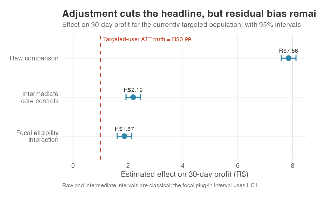
Figure 13.7 summarizes the progression from the raw comparison to the focal estimate. Core controls cut the raw R$7.86 to the intermediate R$2.19, leaving a R$1.20 gap from the targeted-user truth. The focal eligibility interaction lowers the observational contrast standardized to targeted users to R$1.87 and the gap to R$0.88. The change is informative, but the focal rechecks and sensitivity benchmark still challenge a causal interpretation.
Put the results into the credibility memo in Table 13.2. It gives stakeholders a one-page summary they can read without rerunning the code. Each row answers a question a careful reader would ask using numbers from the checks above.
| Memo line | What the evidence says |
|---|---|
| Estimate and estimand | Focal observational contrast standardized to the targeted-user population: R$1.87 [R$1.60, R$2.13]. It targets the treated-user population but does not identify the ATT. The targeted-user ATT truth is R$0.99 in this simulation; the raw comparison is R$7.86 and the intermediate core-controls result is R$2.19. |
| Identifying assumptions | A causal interpretation of the targeted-user contrast requires a well-defined and consistently measured exposure, no spillovers, conditional comparability after the eligibility interaction and core controls, adequate overlap over the treated-population support, and correctly specified outcome and treatment-effect models. In this simulation, hidden shopping_intent violates comparability and biases the observational contrast upward. In an applied analysis, latent intent would remain a hypothesized threat. |
| Focal falsification results | Placebo in time: R$1.60 [R$1.33, R$1.88]. Negative-control outcome: R$1.13 [R$0.96, R$1.29]. Score-preserving fake exposure: R$1.38 [R$1.02, R$1.73]. Each violates its focal zero implication. |
| Robustness results | Core controls, context covariates, and trimming stay near R$1.865. Score adjustment, IPW, and matching fall between R$1.08 and R$1.22. The estimate changes when the analysis uses the targeting process more directly. Even IPW remains 23% above the simulated targeted-user truth of R$0.99, and its two tested placebos remain nonzero. |
| Sensitivity result | In the classical model, a confounder with a partial \(R^2\) of 7.7% with both residual treatment and residual outcome could reduce the estimate to zero (RV 0.077); 6.7% could make it nonsignificant at the 5% level (RV 0.067). The treatment term has a partial \(R^2\) of 0.0065 with the outcome, so it is associated with 0.65% of residual outcome variation after the other model terms. In this simulation, adjustment for the actual hidden factor gives R$0.91 [R$0.64, R$1.17]. A separate worst-case benchmark based on prior_profit gives R$-1.19 [R$-1.44, R$-0.94]. Neither number is a predicted correction. |
| Remaining threats | Known in this simulation: hidden shopping_intent. In an applied analysis: unmeasured intent, functional-form or measurement error, and the inability of a targeted-user ATT to identify effects for currently untreated users. |
| Recommendation | Do not use this observational contrast to authorize whole-base rollout. Run a randomized holdout among current targets to learn whether to continue today’s policy, and include currently untreated users if the decision is expansion to the whole base. |
The memo does not say the banner has no effect. In the simulation, the targeted-user truth is R$0.99, the eligible-targeted truth is R$1.50, and the whole-base truth is R$0.90. It says the focal observational contrast remains too vulnerable for a confident causal claim. Standardizing to targeted users defines the population; it does not identify the ATT or answer the rollout question for currently untreated users.
Key takeaway. The memo makes the target population explicit, relies on the focal rechecks, and separates continuation of current targeting from whole-base rollout. Both decisions need randomized evidence, but the expansion decision must include the currently untreated population.
13.9 Wrapping up and next steps
Credibility comes from stating implications that can fail and reporting what happened when you checked them. An estimate that has never been challenged is untested, and untested is not the same as sound.
The chapter’s main lessons are practical:
- Name the assumption — and the direction bias would take if it fails.
- Look where the effect should be zero, and preserve the parts of the main analysis that carry the problem.
- Judge power before reading the point estimate; a null result with a wide confidence interval offers little reassurance.
- Change one thing at a time, and report test by test — never average the spread away.
- Bound what you cannot test; a fragile result deserves a fragile-sounding conclusion.
- List competing causes, test whether the pattern is specific to the mechanism, and seek evidence built on a different assignment mechanism.
- Report what survived and what did not, and pre-specify so you are not grading on a curve you drew after the fact.
Use those habits in this order:
- Define the estimand, target population, decision, and identifying assumption before you inspect the diagnostics.
- Pre-specify placebo checks, their no-effect-by-construction logic, and the smallest failure that would change the decision.
- Preserve the focal estimand and design logic, judge power, vary one defensible choice at a time, and benchmark hidden confounding.
- Put the estimate, failures, surviving checks, unresolved threats, and next action into a one-page credibility memo.
On the banner, core controls pull the raw R$7.86 to the intermediate R$2.19. The focal observational contrast standardized to targeted users is R$1.87 [R$1.60, R$2.13], still R$0.88 above the targeted-user truth R$0.99. The focal placebos remain nonzero, and the formal 1× prior_profit bound gives a worst-case coefficient of R$-1.19 [R$-1.44, R$-0.94]. The next step is a randomized holdout designed for the decision: current targets for continuation, and currently untreated users for whole-base rollout.
These steps connect to two earlier chapters. The DAG in Section 6.4.2 can imply observable restrictions, but each statistical check also carries modeling assumptions. Balance and planning (Table 3.1, Section 3.4.3) apply the same skeptical habit before estimation. Once an estimate does survive these checks, the next chapter asks what it is worth: what the effect becomes after you discount it for decay, adoption, and the cost of shipping the change.
13.10 Appendix: advanced sensitivity and specification tools
The chapter body covers the tools used in most analyses. This appendix collects less common methods and the formal reasoning behind several choices made above. Each entry gives enough guidance to decide whether a method fits; follow the citation for a full treatment.
The c-dependence breakdown point. Partial-\(R^2\) sensitivity analysis asks how strong an omitted confounder would have to be to change the result within a linear model. Masten and Poirier instead relax conditional independence by an amount \(c\). Here, \(c\) is the largest permitted difference between the treatment probability conditional on observed covariates and a potential outcome, \(P(X=1 \mid Y_x, W)\), and the ordinary propensity, \(P(X=1 \mid W)\). The breakdown point is the smallest value of \(c\) at which a stated conclusion, such as the sign of an effect or a confidence-set claim, no longer holds (Masten and Poirier 2018, 2020).
The cited sources document Stata tooling (Masten et al. 2024). Implementing the estimator outside that software requires the source’s first-step models for the propensity score and conditional quantiles, followed by its bound and inference procedure. A generic grid with a bespoke bootstrap is not equivalent. For the applications in this chapter, start with partial-\(R^2\) sensitivity analysis; use c-dependence when its linear sensitivity model is the concern.
Specification-curve and multiverse analysis. The six-row grid in the robustness section is a hand-built version of a larger idea. When defensible choices multiply, estimate the effect under their pre-declared combinations and plot the distribution rather than selecting one preferred path. A specification curve orders estimates by size (Simonsohn et al. 2020); multiverse analysis extends the choice set through the cleaning and coding pipeline (Steegen et al. 2016). In R, specr builds the curve; in Python, a loop over the choice grid can do the same. Pre-register the choice set and report the curve rather than cherry-picking a point (Section 3.1).
The likelihood-ratio reading of a placebo. The asymmetry this chapter repeats — a fired placebo is evidence against its maintained implication, while a null one offers limited support — has a formal interpretation. Eggers, Tuñón, and Dafoe frame a placebo result as a likelihood ratio that shifts belief rather than a verdict that settles it (Eggers et al. 2024). A fired placebo is more likely when the tested implication fails than when it holds, so it shifts belief against that implication. How much a placebo estimate near zero strengthens confidence that the true placebo effect is zero depends on the test’s power. If the test is underpowered, a near-zero estimate provides little evidence that the true placebo effect is zero.
Equivalence testing for a “passing” placebo. A non-significant placebo is not proof of no effect; it can simply be underpowered, the wide-CI null the body warned about. The disciplined reframe is an equivalence test. Pre-declare a margin you would consider negligible, then use the confidence interval or formal equivalence test to rule out placebo effects at or beyond that margin (Hartman and Hidalgo 2018). An informative equivalence result means “bounded near zero”; do not call a merely non-significant placebo a pass. The same distinction applies to a balance table. An SMD below a rule-of-thumb threshold is a descriptive diagnostic; a formal equivalence test asks whether each covariate difference is estimated precisely enough to rule out magnitudes larger than a negligible margin specified in advance (Section 13.4.5).
Further practice. To see what each diagnostic detects, change the data-generating process in this chapter’s R companion script, write the result to a scratch path of your own, and point the chapter’s R or Python analyses at that copy. The companion keeps its write_csv() lines commented out on purpose: overwriting data/free_shipping_banner.csv would break every number printed in this chapter. Increase the effect of hidden shopping_intent: the placebo-in-time and negative-control estimates should move farther from zero, the balance gap should widen, and the Robustness Value should fall. Remove shopping_intent: the placebo estimates should move toward zero, balance should improve, and the Robustness Value should rise. Repeating the exercise shows which part of the data-generating process drives each diagnostic.
External resources. For more worked placebo examples, see Chabé-Ferret’s chapter on falsification (Chabé-Ferret 2025); for the practitioner’s case for purposeful robustness, Huntington-Klein’s essay (Huntington-Klein 2021); and for the sensitivity tooling, the sensemakr paper and documentation, with the Python implementation at PySensemakr (Cinelli, Ferwerda, et al. 2024; LaPierre 2024).
Key takeaway. The body’s tools cover most analyses; use these methods for narrower problems. Use the breakdown point when linearity is the concern, a specification curve when there are many defensible analytic choices, equivalence testing when a “passing” placebo must mean bounded near zero, and the likelihood-ratio framework to judge reassurance in light of test power.
As Google advises, “NotebookLM can be inaccurate; please double-check its content”. I recommend reading the chapter first, then listening to the audio to reinforce what you’ve learned.↩︎
To load it directly, use the example URL
https://raw.githubusercontent.com/RobsonTigre/everyday-ci/main/data/free_shipping_banner.csv.↩︎This book deliberately stops short of teaching propensity-score matching as a complete method. Its causal interpretation requires conditional exchangeability given the observed covariates and adequate overlap. Proper implementation also requires decisions about the covariates and treatment model used to estimate the score; the matching algorithm, caliper, and replacement; the target estimand; balance and overlap diagnostics; outcome analysis and uncertainty; and sensitivity to hidden bias. The book has not developed the treatment-modeling and design-validation machinery needed to cover those choices responsibly, so estimating a score and calling a matching function is not enough. Because the method remains widely used, the example below introduces the workflow without serving as an implementation template. For practical guidance, see Caliendo and Kopeinig (2008), Stuart (2010), and Austin (2011).↩︎
The calculation ships as
sensemakrin R andPySensemakrin Python (Cinelli, Ferwerda, et al. 2024; LaPierre 2024). The Python package installs asPySensemakrbut imports assensemakr. Its ownplot()helper breaks on matplotlib 3.10 and later, so the Python block below draws the contour from the package’s bias functions instead; R’splot(sens)still works.↩︎A SKU identifies one sellable product variant, such as a blue running shoe in size 42; size 43 is another. Prices and stock are set at this level, so one popular SKU can move category sales.↩︎