graph LR
    Z["Z (Instrument)"]
    D["D (Treatment)"]
    Y["Y (Outcome)"]
    U["U (Unobserved)"]
    X["X (Covariates)"]

    U -.-> D
    U -.-> Y
    X --> D
    X --> Y
    D --> Y
    Z --> D

    style U stroke-dasharray: 5, 5
    linkStyle 5 stroke-width:4px,stroke:magenta
7 Instrumental variables: When people don’t do what they were assigned to
Keywords
A/B Testing, Causal Inference, Causal Time Series Analysis, Data Science, Difference-in-Differences, Directed Acyclic Graphs, Econometrics, Impact Evaluation, Instrumental Variables, Heterogeneous Treatment Effects, Potential Outcomes, Power Analysis, Sample Size Calculation, Python and R Programming, Randomized Experiments, Regression Discontinuity, Treatment Effects
7.1 When people don’t do what you assigned them to do
In Chapter 4, we assumed everyone assigned to the treatment group actually received the treatment, and everyone in the control group didn’t. This is called perfect compliance.2 It’s a scenario that makes our lives as data-people much easier.
But reality has other plans. In the real world, you can randomly assign people to receive an offer, an invitation, or access to something, but you can’t force them to actually use it. This is called imperfect compliance, meaning people don’t always do what they were assigned to do. Consider these common scenarios in tech and digital businesses:
- You send discount coupons to randomly selected customers, but not everyone redeems them;
- You offer a free trial of a premium feature to half your users, but many never activate it;
- You launch a new onboarding tutorial for new app users, but some skip it entirely;
- You invite customers to join a paid membership program, but participation is voluntary.
This is the world of imperfect compliance, and it’s everywhere. In my experience, most of the interventions listed above don’t get more than 10% of users to take the desired action. Some achieve adoption rates below 5%. But even with low adoption, the business should learn the impact of the intervention on those who actually took it.
That information is input for strategy: if the effect is substantial for those users who took the intervention, it may make sense to invest in increasing adoption (e.g., better marketing about the free trial, better copy and UX for the discount coupons). If the effect is minimal even among those who did what you asked, it might be time to kill the promo or feature entirely.
The good news is that instrumental variables (IV) methods give us a rigorous way to estimate these causal effects even when compliance is imperfect. Better yet, you’ve already learned most of the concepts you need to apply IV methods.
Learning through example: email frequency optimization
Instrumental variables can be intricate because of the many logical steps involved. To avoid losing track, I’ll use a running example to guide us.
Let’s ground this in a concrete example we’ll use throughout the chapter. Imagine you work at an e-commerce company that currently sends promotional emails to customers once a week — we’ll call this the Business as Usual (BAU) scenario, corporate shorthand for the status quo.
Your marketing team believes that switching to daily emails featuring curated “daily deals” (often marketed as “hidden gems” or “great finds”) could increase revenue. However, they’re also concerned that this higher frequency might annoy customers and drive up unsubscribe rates, causing more harm than good. To settle the debate, you decide to run an experiment.
A workaround is to offer users the option to switch to daily emails. This is a common strategy in tech and digital businesses, which is the basis for what we call “encouragement design”. The problem is that if you simply compare those who opt-in against those who don’t, even those in the control group, you’re not measuring the effect of emails — you’re measuring the enthusiasm of your engaged users.
So your solution is to randomly split customers into two groups:
Treatment group, usually denoted in a dataset by \(Z=1\) (50% of all users): Receives a friendly email invitation: “Want to hear from us more often? Switch to daily deals!” with a one-click opt-in button.
Control group, usually by \(Z=0\) (50% of all users): No invitation. They stay on weekly emails by default, though they could manually change preferences if they discover the setting.
Here’s where imperfect compliance comes in. Not everyone who gets the invitation will switch to daily emails, denoted by \(D=1\). This creates a gap between who you assigned to get the treatment (receiving the invitation) and who actually receives the treatment (enabling daily emails).
This chapter will show you how to estimate the causal effect of daily emails in this realistic scenario.
NoteNotation for this chapter
Let’s agree on the interchangeable use of some names for our variables throughout this chapter’s formulas and code:
- \(Y \rightarrow\)
revenue: The outcome variable (60-day user-generated revenue). - \(Z \rightarrow\)
invitation: The instrument (random assignment to receive the specific invitation email). - \(D \rightarrow\)
daily_emails: The treatment (actually receiving/opt-in to daily emails).
7.2 Some ways to measure effects with imperfect compliance
When compliance is imperfect, we have two main estimands, or target quantities, that we can measure.3 Understanding the difference between them is essential for interpreting your results correctly.
The Intention-to-Treat (ITT) answers the policy question: “What is the impact of offering this program to everyone?” The Local Average Treatment Effect (LATE) answers the efficacy question: “What is the impact on the specific group of people who actually participated because of the offer?”4
7.2.1 Intention-to-treat (ITT): the effect of the offer
The intention-to-treat effect measures the impact of being assigned to receive the treatment, regardless of whether people actually use it. In our email example, ITT compares the revenue of everyone who got the invitation (treatment group) with everyone who didn’t (control group).
The key advantage of this causal metric is that it preserves the beauty of randomization. Because group assignment was random, any difference in outcomes between the groups must be causal. However, ITT typically gives you a conservative estimate because it mixes together:
- People who switched to daily emails because of your invitation (and potentially benefited)
- People who got the invitation but didn’t switch (and experienced no effect)
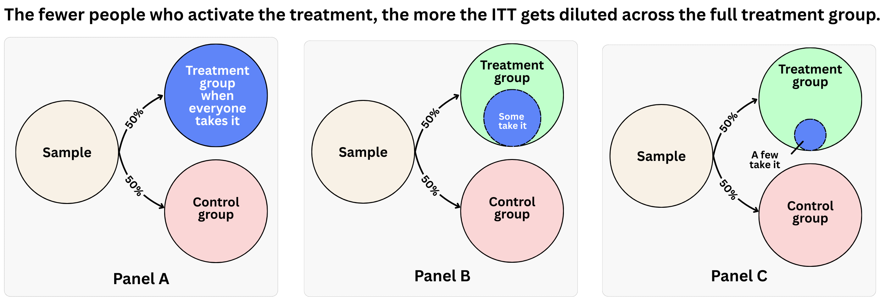
This creates dilution, as illustrated in Figure 7.1. Even if the effect of daily emails is huge for those who actually receive them, this effect will be diluted over the whole treatment group in case only a small portion of the invited group switches. In such cases, the ITT might be small, and the analyst will learn nothing about how the treatment worked out for those who took advantage of it.
Think of ITT as answering: “What’s the effect of offering this treatment to everyone?” This is useful when you’re deciding whether to roll out a program, but it obscures the efficacy of the treatment itself. For additional visualizations and a simulated example showing how imperfect compliance affects the interpretation and statistical power of experiments, see Section 5.4.5.
7.2.2 Understanding compliance and the Local Average Treatment Effect
To understand what Instrumental Variables estimates, we first need to formalize the types of non-compliance. This gap between assignment (\(Z\)) and actual treatment (\(D\)) happens in two ways:
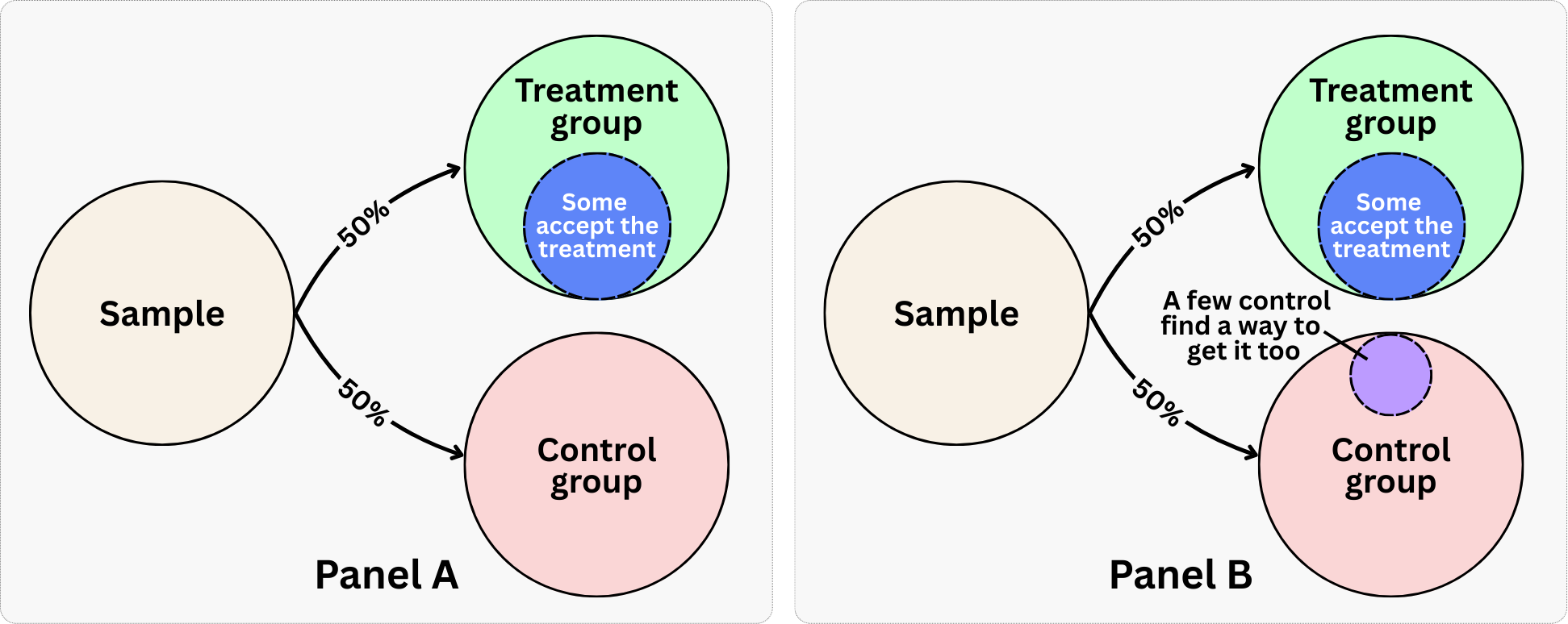
One-sided non-compliance: Users assigned to the control group cannot access the treatment (so they never take it), but users assigned to the treatment group can choose to decline it. This is common in the business cases we mentioned previously. Panel A of Figure 7.2 illustrates this scenario: notice how the control group remains “pure” (no one gets treated), while within the treatment group only some users accept the intervention.
Two-sided non-compliance: Non-compliance happens on both ends. Some treated users decline the treatment, AND some control users manage to access the treatment anyway. Panel B of Figure 7.2 shows this pattern: beyond the partial uptake in the treatment group, “a few control find a way to get it too.” In our email example, a few control users might stumble upon a “Switch to daily emails” toggle buried deep in their account settings and opt in on their own, without ever receiving an invitation.5
To make sense of this, we categorize the population into four types of people based on how they react to the assignment (see Imbens and Rubin 2015, Ch. 23-24):
Compliers (“the persuadables”): These people do what they are told. They take the treatment if assigned to it (\(Z=1 \rightarrow D=1\)) and don’t take it if assigned to control (\(Z=0 \rightarrow D=0\)). The IV method estimates the Local Average Treatment Effect (LATE), which is specifically the treatment effect for this group.
Always-takers (“the enthusiasts”): They always take the treatment, regardless of assignment (\(D=1\) irrespective of \(Z\)). Even if they are in the control group, they find a way to get treated.
Never-takers (“the unreachables”): They never take the treatment, regardless of assignment (\(D=0\) irrespective of \(Z\)). Even if you send them the invite, they ignore it.
Defiers (“the contrarians”): They do the opposite of what is assigned. If assigned treatment, they refuse; if assigned control, they take it. We typically assume defiers don’t exist — the monotonicity assumption, formalized in Section 7.4.4 below.
Why “local” average treatment effect?
LATE is called “local” because it only applies to compliers, not the entire population. This is both a strength and a limitation. On one hand, compliers are the persuadable segment, exactly the users you can influence through better marketing or product design. On the other hand, compliers may be systematically different from the rest of your users.
They might be more engaged, more price-sensitive, or more responsive to communications. If you roll out daily emails to everyone based on the LATE (as we’ll see in the application below, approximately R$13.6), the effect for always-takers and never-takers could be quite different (or even negative). LATE tells you the treatment works for those you can persuade; it doesn’t tell you what happens when you stop asking and start mandating.
In this chapter, we illustrate the method with a scenario of two-sided non-compliance. This is realistic for digital products: even without receiving an invitation, some users in the control group might stumble upon a setting to activate the feature while browsing their account, or hear about daily deals from a friend who did get invited. These are the always-takers, which defines two-sided non-compliance.
7.2.3 Why not just compare those who took the treatment?
You might be tempted to ask: “If we know who actually switched to daily emails in the treatment group, why don’t we just compare them to the control group?” Or perhaps, “Why not compare them to the people in the treatment group who didn’t switch?”
These approaches are dangerously misleading. (In medical research, they are called “as-treated” analyses, but the logic is the same.) Recent work by Angrist et al. (2025) and Angrist and Hull (2023) highlights how these naive comparisons destroy the benefits of randomization and reintroduce selection bias.
Here is the problem: in the treatment group, the people who switch to daily emails (the compliers) are likely different from those who don’t. They might be more engaged, more loyal, or simply more curious. These are characteristics that also drive revenue.
If you compare these “enthusiastic switchers” (\(D=1\)) to the entire control group, you are comparing a select group of high-potential users against a mix of high-potential and low-potential users. The result? You will overestimate the effect of daily emails because you are conflating the effect of the emails with the effect of being an enthusiastic user.
Ideally, you would want to compare compliers in the treatment group with would-be compliers in the control group. But here lies the fundamental issue: we cannot see who the compliers are in the control group. Most people in the control stay on weekly emails, aside from a small fraction of always-takers who switch on their own. But among those who stayed on weekly, we don’t know who would have switched if they had been offered the invitation.
The compliers in the control group are invisible to us, mixed in with never-takers who also stayed on weekly emails. We can rule out defiers, “the contrarians”, thanks to the monotonicity assumption (discussed below), but we still can’t tell compliers apart from never-takers. Without that distinction, there’s no direct “apples-to-apples” comparison. This is precisely why Instrumental Variables exist: the method leverages random assignment to mathematically isolate the causal effect for compliers, even though we never observe who they are.
7.3 How instrumental variables work
Now that we understand what we’re trying to estimate, let’s see how IV methods actually work. The mechanics of IV use randomization in a clever way to isolate the causal effect for compliers, even though we can never directly identify who the compliers are in our data.
The IV approach breaks down the problem into three steps, which we can think of as three different effects:
7.3.1 The reduced form effect (ITT): from the assignment to the outcome
This is the simplest step. We just compare the average outcome for everyone assigned to treatment versus the average outcome for everyone assigned to control. In our email example:6
\[ITT = \text{avg}(\text{revenue}_i | \text{invitation} = 1) - \text{avg}(\text{revenue}_i | \text{invitation} = 0)\]
This tells us: “What’s the overall effect of sending the invitation on revenue?” It’s also called the “reduced form” effect, because it’s the effect of the instrument (invitation) on the outcome (revenue) without worrying about the intermediate step of actually switching to daily emails.
If everyone who was assigned to the treatment clicked the opt-in button, we would be in a scenario of perfect compliance — where assignment (\(Z\)) perfectly predicts treatment receipt (\(D\)). In that case, the ITT would also be the Average Treatment Effect (ATE), because the intention of this e-commerce to send daily emails to those users became reality for all of them.
7.3.2 The first stage effect: from the assignment to the treatment uptake
In our example, the first stage effect is the difference in the proportion of people receiving daily emails between those who got the invitation (treatment group) and those who didn’t (control group):
\[\text{First stage} = \text{avg}[\text{daily\_emails}_i | \text{invitation} = 1] - \text{avg}[\text{daily\_emails}_i | \text{invitation} = 0]\]
This tells us: “How much does the invitation increase the probability of opting-in to daily emails?” It’s called “first stage” because it’s the first link in the chain reaction invitation → daily_emails → revenue. A strong first stage is essential for IV to work well, as we’ll see next.
Why it matters: If your instrument doesn’t actually nudge people toward treatment, you have nothing to work with. The first stage tells you whether the bridge exists. It measures how effective your instrument is at changing treatment status.
7.3.3 The Wald estimator: from diluted to local effects
The core idea is simple: divide the overall effect of the invitation (ITT) by the fraction of people whose behavior it changed (the first stage). This scales up the diluted effect back to the true effect for compliers. For the formal mathematical decomposition, see the Appendix 7.A:
\[ \begin{aligned} \text{LATE} &= \frac{\text{ITT}}{\text{First stage}} \\[0.5em] &= \frac{\text{avg}[\text{revenue}_i | \text{invitation}_i = 1] - \text{avg}[\text{revenue}_i | \text{invitation}_i = 0]}{\text{avg}[\text{daily\_emails}_i | \text{invitation}_i = 1] - \text{avg}[\text{daily\_emails}_i | \text{invitation}_i = 0]} \\[0.5em] &= \frac{\text{Effect of receiving the invitation on revenue}}{\text{Effect of receiving the invitation on opting in to daily emails}} \end{aligned} \]
As we saw in the discussion on ITT, the effect of the invitation on revenue (the numerator) is called the reduced form effect. The denominator is the first stage: the effect of receiving the invitation on opting in to daily emails.
Here’s a concrete example with numbers (matching the simulation we’ll run shortly):
- ITT, the effect of the invitation on revenue ≈ R$4.2 (revenue increases by about R$4.2 on average for everyone assigned to the invitation).
- First stage, the effect of the invitation on opting in to daily emails ≈ 0.31 (the proportion receiving daily emails is 31 percentage points higher in the treatment group than in the control group: 0.36 - 0.055).
- LATE = R$4.2 / 0.31 ≈ R$13.6 (the effect of daily emails on revenue for compliers).
This tells us that for compliers (those who switched because of the invitation), daily emails increase revenue by about R$13.6. The effect is larger than ITT because we’re no longer averaging over the non-compliers who received zero effect.
Now you can see why a strong first stage matters. Since LATE = ITT / First stage, a tiny first stage means you’re dividing by a number close to zero. Imagine if 6% of invited users switched to daily emails but 5% of control users also found their way to the setting on their own — the first stage is just 0.06 - 0.05 = 0.01. With an ITT of R$5, you’d get LATE = R$5 / 0.01 = R$500. This is the “weak instrument” problem. It causes two kinds of trouble.
First, your estimates become wildly unstable — small fluctuations in the data produce huge swings in your LATE. Second, and more insidiously, weak instruments bias your estimate toward the naive OLS comparison you were trying to avoid. A tiny denominator amplifies not just the true signal but also any residual confounding in the numerator, pulling your LATE toward a simple comparison of daily email users vs. non-users, selection bias included.
You’re not just getting a noisy answer; you’re getting an answer contaminated by the very confounding you designed the instrument to eliminate. We’ll return to testing for instrument strength shortly. For now, keep in mind that a strong first stage keeps your estimate both stable and on the right track.
7.3.4 Two-stage least squares: from the Wald estimator to regression
The Wald estimator gives us the intuition, but in practice we use a technique called two-stage least squares (2SLS). As the name suggests, it involves running two regressions: one to predict treatment from the instrument, and another to estimate the treatment effect using those predictions. This approach lets us include covariates and get proper standard errors.
First stage: Regress treatment uptake on the instrument (and covariates)
\[ \text{daily\_emails}_i = \alpha_0 + \alpha_1 \text{invitation}_i + \gamma' X_i + u_i \tag{7.1}\]
Here, \(\alpha_1\) represents the first stage effect: it measures how much the invitation increases the probability of receiving daily emails. We also include \(X_i\), covariates like customer tenure or past purchases. While randomization ensures we don’t need controls to get the right answer, including them may make our estimates more precise, effectively giving us more “power” to detect effects.
As we learned in Chapter 1, fitting a regression model gives us both parameter estimates and fitted values (predictions). In the first stage of 2SLS, we rely on these predictions. We use the model in Equation 7.1 to predict what the user’s opt-in choice would be based solely on the randomly assigned invitation.
This step extracts only the variation in treatment that comes from the instrument. When we use the random invitation (\(Z_i = \text{invitation}_i\)) to predict who opts in (\(\widehat{D}_i = \widehat{\text{daily\_emails}}_i\)), we filter out the user’s personal choice and keep only the part of treatment assignment that was driven by the experiment. What remains is a “clean” version of the treatment, free from the confounding influence of unobserved factors like motivation or loyalty.
Second stage: Regress the outcome on the predicted treatment from the first stage \[\text{revenue}_i = \beta_0 + \beta_1 \widehat{\text{daily\_emails}}_i + \delta' X_i + \varepsilon_i\]
The coefficient \(\beta_1\) is the Local Average Treatment Effect (LATE). It captures the causal effect of daily emails specifically for compliers. By using the predicted treatment values (\(\widehat{\text{daily\_emails}}_i\)) — which are cleansed of self-selection bias — we recover the true causal impact.
Although this plug-in approach of taking the predictions from the first stage to run the second stage gives the correct point estimate for \(\beta_1\) (the LATE), if you run those two regressions like I suggested above, you’ll get wrong standard errors (and therefore misleading confidence intervals and p-values). This is because the second stage ignores that the treatment was estimated in the first stage, and that estimations carry their own noise, uncertainty, and variance.
Proper 2SLS fixes this internally. In practice, you don’t need to implement the correction yourself: the standard 2SLS functions in R and Python run both stages together and report the correct inference.
7.4 Key assumptions for instrumental variables
IV is a set of logical claims stacked on top of each other. For the math to recover a causal effect, we need to believe in some core assumptions. These are the logical links that support our entire causal claim. Let’s walk through them using our email experiment.
7.4.1 Relevance: the instrument must affect treatment
This is the most testable assumption. It ensures there is a bridge between the instrument and the treatment. The invitation must actually change the probability of receiving daily_emails. In statistical terms, our “first stage” must be strong.
In our example: The invitation email needs to be persuasive enough to make a substantial number of customers switch to daily emails. The magenta arrow in Figure 7.3 must be strong. If just a small fraction of people click the opt-in button as a response to the invitation, that bridge is broken, and we can’t learn much about the effect of daily emails.
How to check it: This is the only assumption that is fully testable. Run the first stage regression and check the F-statistic, which measures how strongly the instrument predicts treatment (the Python and R scripts will teach you how). A value above 10 indicates the instrument is strong enough to be useful.7 Visually, you should see a clear jump in daily_emails adoption in the treatment group compared to the control group.
What happens if violated: We have a “weak instrument.” The IV estimates become unstable, standard errors explode, and the results become useless.
7.4.3 Exclusion restriction: no direct effects
This assumption says the instrument can only affect the outcome through the treatment, nothing else. It is often the hardest assumption to defend. It states that the instrument (invitation) affects the outcome (revenue) only through the treatment (daily_emails). In other words, there is no direct arrow from \(Z\) to \(Y\) in the DAG. As shown in Figure 7.5, the only path from the instrument to the outcome must flow through the treatment (the path highlighted in cyan).
How to check it: This is fundamentally untestable with data alone. You need to rely on:
- Strong experimental design (make the invitation email as neutral as possible)
- Institutional knowledge (understand how the system works)
- Placebo tests, where you check if the instrument affects outcomes it logically cannot affect (like revenue from the week before the experiment started; if you find an effect there, something is wrong)8
What happens if violated: The instrument cannot have a life of its own, otherwise the LATE estimate will be biased. You would be attributing to daily emails effects that actually come from other pathways. For example, if the invitation email itself contained a “20% off” coupon, that would drive immediate purchases directly from \(Z\) to \(Y\), bypassing the treatment entirely. Similarly, simply seeing the invitation might make customers feel valued, increasing their loyalty and spending regardless of whether they switch email frequency. Even the act of clicking through to the preference center could expose customers to other products they wouldn’t have seen otherwise, creating another direct link between the instrument and the outcome.
graph LR
    Z["Z (Instrument)"]
    D["D (Treatment)"]
    Y["Y (Outcome)"]
    U["U (Unobserved)"]
    X["X (Covariates)"]

    U -.-> D
    U -.-> Y
    X --> D
    X --> Y
    D --> Y
    Z --> D

    style U stroke-dasharray: 5, 5
    linkStyle 4,5 stroke-width:4px,stroke:cyan
7.4.4 Monotonicity: no defiers
We assume that the instrument pushes everyone in the same direction (monotonicity means moving in only one direction). In other words, there shouldn’t be customers who would switch to daily emails when not invited but stay weekly when invited; the ones we call “defiers,” which we previously nicknamed “the contrarians.”
In our example: It means there are no customers who would switch to daily_emails = 1 if we didn’t invite them (i.e., invite = 0), but would refuse to switch if we did invite them (i.e., daily_emails = 0 if invite = 1). Given that the invitation is a friendly prompt, this is a safe bet.
How to check it: Like the exclusion restriction, we can’t directly test this assumption with data. However, in “encouragement designs” like ours, where the instrument is simply a friendly invitation, monotonicity is usually a safe bet. You verify it by carefully designing your experiment and thinking through all the ways users might react to the invitation.
What happens if violated: The interpretation of LATE breaks down, as “defiers” would subtract from the effect while “compliers” add to it. In other words, it’s no longer an average for compliers but a weighted average of compliers and defiers with opposite-signed effects.
7.4.5 SUTVA: no interference between units
We discussed this assumption in Section 4.1.1.2, and it applies here too. One customer’s treatment status shouldn’t affect another customer’s outcomes, and there shouldn’t be multiple versions of treatment.
In our example: This would be violated if: - Customers share deals from emails with each other, affecting revenue for people not receiving daily emails - Daily email recipients buy up limited inventory, reducing what’s available for others - There are different types of daily emails (some promotional, some informational) that have different effects
How to check it: Think carefully about potential spillover effects based on how your platform works. If you’re worried about interference, consider using clustered randomization (e.g., randomize at the household or geographic level).
What happens if violated: Your estimates may be biased, and standard errors may be wrong. The direction of bias depends on whether spillovers are positive or negative.
WarningThe credibility hierarchy
Among these assumptions, relevance is the easiest to check (just look at the first stage), SUTVA and monotonicity are often made plausible by the design of the study, but exclusion restriction is the hardest to guarantee. This is why careful experimental design is essential. Make sure your instrument is as clean as possible, affecting treatment uptake without directly influencing outcomes.
One more validity check: Beyond the core assumptions, consider whether differential attrition is a concern — we introduced this in Chapter 4. Hover your mouse over Figure 4.4 to recall the issue. Higher-frequency emails may cause some users to unsubscribe entirely, exiting your measurement window. If these “annoyed” users disproportionately leave the treatment group, your outcome data will be measured only on survivors: users who tolerated daily emails.
This survivorship bias can make your LATE look more positive than it truly is. To guard against this, track unsubscribe rates between treatment and control groups and consider whether unsubscribers should be included in your analysis (perhaps with imputed outcomes or as a separate outcome variable).
7.5 Application: does daily email frequency increase revenue?
Tip💻 Want to run the code? Set up your environment: click here
Data: All data we’ll use are available in the repository. You can download it there or load it directly by passing the raw URL to read.csv() in R or pd.read_csv() in Python.9
Packages: To run the code yourself, you’ll need a few tools. The block below loads them for you. Quick tip: you only need to install these packages once, but you must load them every time you start a new session in R or Python.
# If you haven't already, run this once to install the packages:
# install.packages(c("tidyverse", "AER", "fixest"))

# You must run the lines below at the start of every new R session.
library(tidyverse)  # Data manipulation and visualization
library(AER)        # For IV regression (ivreg function)
library(fixest)     # For OLS with robust standard errors (feols function)
# If you haven't already, run this in your terminal to install the packages:
# pip install numpy pandas statsmodels linearmodels matplotlib
# You must run the lines below at the start of every new Python session.
import numpy as np # Mathematical computing
import pandas as pd # Data manipulation
import statsmodels.api as sm # Statistical models
import statsmodels.formula.api as smf # Formula-based regression
from linearmodels.iv import IV2SLS # Two-stage least squares for IV
import matplotlib.pyplot as plt # VisualizationNow for the test: I’m going to walk you through the same email frequency experiment we’ve been discussing, but with numbers. I simulated 10,000 customers who went through our experiment. Half received the invitation (invitation = 1) to switch to daily emails (daily_emails), half didn’t (invitation = 0). The outcome is revenue over a 60-day window, measured in R$ (revenue).
Here’s the twist that makes this interesting: I know the ground truth. When I built the simulation, I set the true treatment effect at R$15 per customer. So we can check whether IV actually recovers the right answer, or whether we’ve been fooling ourselves with fancy math.
But first, let’s acknowledge something uncomfortable. We don’t have perfect compliance. In the simulation, only about 36% of invited customers clicked that opt-in button. Meanwhile, 5.5% of customers who never got an invitation found the setting on their own and switched anyway (our always-takers). This is messy, realistic data.
Here’s the second twist: the simulation includes an unobservable variable that we, as analysts, cannot see (in the R and Python scripts you can see how I created it). This variable represents something like “user enthusiasm” or “deal-seeking propensity.” It drives both who opts into daily emails and who spends more money. This creates a trap for the unwary analyst.
If you simply compare revenue between those who received daily emails versus those who didn’t (the “as-treated” approach), you’ll get a biased estimate. I encourage you to run the full code and compare the as-treated estimate to the LATE at the end.10 You’ll find that the naive approach overestimates the effect by about 25% because it conflates the true treatment effect with the selection effect of enthusiastic users.
The question is: can we still learn something useful?
Step 1: Does the bridge even exist?
Before we estimate any treatment effects, we need to answer a more fundamental question: does the invitation actually change behavior? If sending the invitation doesn’t make people more likely to switch to daily emails, then the whole IV approach falls apart. We’d be dividing by something close to zero, and our estimates would be meaningless.
This is the relevance assumption, and unlike the other IV assumptions, we can test it directly. Let’s see what the data tells us.
The results are encouraging. The invitation increases the probability of switching to daily emails by about 31 percentage points (36% in the treatment group vs. 5.5% in control). That’s a substantial effect, and the F-statistic is well above 10, so we can rule out the weak instrument problem. The bridge exists, and it’s sturdy enough to walk across. Now let’s see what happens when people walk across it.
Step 2: What’s the overall policy effect (ITT)?
Now let’s answer the question any marketing director would ask: “If we send this invitation to everyone, how much extra revenue can we expect?”
This is the intention-to-treat (ITT) effect. It’s the simple, clean comparison between everyone who got the invitation and everyone who didn’t. No correction for who actually switched, no adjustment for compliance. Just “Did sending the invitation make money?”
The answer: about R$4.2 per customer. Statistically significant — a promising start. Recall the effect per customer who opts-in to daily emails because of the invitation is R$15. Why is our estimate so much smaller?
This is the dilution problem in action. Only about a third of invited customers actually switched to daily emails. The other two-thirds received the invitation, shrugged, and kept their weekly emails. For them, the invitation had no effect whatsoever. When we average across everyone who got the invitation, including all those shrugging non-compliers, the effect gets watered down.
The R$4.2 ITT isn’t wrong. It’s the right answer to a different question: “What’s the average effect of sending this invitation?” If that’s all you care about, for instance, for a simple ROI calculation, you’re done here.
But if you want to know whether daily emails actually work for people who receive them, we need to dig deeper.
Step 3: Uncovering the true effect for compliers
Now comes the moment of truth. We’re going to use instrumental variables to strip away the dilution and recover the effect of daily emails for people who actually switched because of our invitation.
Recall: LATE = ITT / First Stage. With actual numbers:
\[ \text{LATE} = \frac{\text{R\$4.2}}{0.31} \approx \text{R\$13.6} \]
Intuitively, we’re “scaling up” the diluted effect to account for the fact that only a third of invited customers actually got the treatment. Sure enough, the LATE estimate comes out to approximately R$13.6, remarkably close to our ground truth of R$15.11 This is the payoff. We started with messy data where only a third of people did what we asked, and we still recovered the true causal effect. The math actually works.
LATE vs. as-treated: Before moving on, I encourage you to run the full simulation code from the book’s repository. Compare the two approaches side by side:
IV/2SLS (LATE): R$13.6, with a 95% confidence interval of roughly [8.97; 18.25]. This interval comfortably contains the true treatment effect of R$15.
As-treated (naive, comparing those who took treatment vs. those who didn’t): R$18.7, with a 95% confidence interval of roughly [16.96; 20.53]. This interval excludes the true value of R$15 entirely.
The naive approach overestimates the effect by about 25%. Worse, its confidence interval is tighter, giving a false sense of precision while pointing in a confidently wrong direction. This is selection bias made visible: the as-treated estimate isn’t just noisy — it’s systematically biased upward because it conflates the true effect of daily emails with the spending habits of enthusiastic users who self-selected into treatment.
Sanity checks: Did we get lucky?
Before declaring victory, let’s run two sanity checks that any skeptic should demand.
Does the estimate change when we add covariates? In a properly randomized experiment, it shouldn’t change dramatically. We ran the IV model twice, once with covariates like tenure_months and past_purchase, and once without. The estimates are nearly identical. This stability is reassuring. If our estimates had swung wildly depending on which controls we included, that would suggest something was wrong with our randomization.
Does the invitation predict things it shouldn’t? Here’s a clever test: let’s see if the invitation predicts customers’ past purchases, before they ever received it. Logically, a future email can’t travel back in time and change history. If we found a significant relationship, it would mean our randomization somehow failed. We’d have accidentally invited customers who were already high spenders.
The placebo test shows exactly what we want: a coefficient close to zero with a p-value well above 0.05. Our instrument is clean.
7.5.1 Business insights to share with stakeholders
We’ve done the statistical work. Now comes the harder part: translating these numbers into decisions. Here’s how to think about each estimate and, equally important, how to avoid common mistakes when presenting them.
Two estimates, two different questions
I’ve repeated that enough times that it’s become a mantra: The ITT and LATE answer fundamentally different business questions. Mixing them up is one of the most common mistakes I see in practice.
| Estimate | Value | Question it answers | Use it for |
|---|---|---|---|
| ITT | R$4.2 | “What happens if we offer this to everyone?” | ROI calculations, forecasting, budget decisions |
| LATE | R$13.6 | “Does the feature work for people who use it?” | Product decisions, understanding mechanisms, prioritization |
The ITT (R$4.2) is your planning number. If you send this invitation to 100,000 customers, you can expect about R$420,000 in incremental revenue. This already accounts for the fact that most people will ignore your invitation. Use this for cost-benefit analysis: if the invitation costs R$1 per customer to send (design, email infrastructure, opportunity cost), your net gain is R$3.2 per customer. That’s a 320% return, and it’s a real, achievable number. Don’t worry much about this business math, I’ll cover it in Chapter 13.
The LATE (R$13.6) is your product signal. It tells you the feature works well for the persuadable segment. If you’re deciding whether to invest in better email content, personalization, or making the daily email setting more discoverable, this is the number that matters. A R$13.6 per-user effect is substantial and justifies further investment in the feature itself.
What the compliance rate tells you
The 36% compliance rate isn’t just a number to plug into a formula. It’s a diagnostic that reveals important information about your product funnel. What counts as “high” or “low” compliance depends entirely on context. Industry benchmarks illustrate this: email open rates average around 43.5% across industries (MailerLite 2025), while a good free-to-paid conversion rate for SaaS products is typically around 8-12% (Rachitsky 2023). Getting 12% of users to convert on a free trial would be strong performance; getting only 12% to open an email would be sad. The same number tells a different story depending on the baseline expectation for your product.12
The gap between ITT and LATE. When compliance is high, ITT and LATE converge because the “dilution” from non-compliers is small. When compliance is low, the gap widens, and specific diagnostics emerge. A low ITT paired with a high LATE may signal a “hidden gem”: the feature is powerful for those who use it, but your invitation isn’t getting enough people through the door (a marketing problem).13 A low ITT paired with a low LATE signals a “dud”: even the people who use the feature don’t see much benefit in terms of the analyzed outcome (a product problem).
How actionable is the finding? High compliance means there’s little room to improve conversion; focus instead on the feature itself. Low compliance suggests untapped potential. Not everyone who ignored your invitation is a true never-taker. Some might be “reachable non-compliers” who would respond to a better prompt, different timing, or clearer value proposition. Consider A/B testing the copy and the channel of the invitation before scaling up.
When to worry about weak instruments. If compliance is very low relative to your baseline, your first-stage effect shrinks, and your LATE estimates become noisy. The F-statistic (which we discussed earlier) will flag this: F < 10 signals trouble. Before trusting a LATE from a weak first stage, invest in understanding why compliance is low. Is the invitation buried? Is the ask too big? You might learn more from qualitative research than from running a larger experiment with the same weak instrument.
Common mistakes to avoid
Presenting LATE as if it applies to everyone. As we discussed earlier, the R$13.6 effect is for compliers only. If you tell stakeholders “daily emails increase revenue by R$13.6 per customer” and then roll out daily emails to everyone, you’ll be disappointed. Always-takers and never-takers won’t respond the way compliers did.
Using ITT when you should use LATE (or vice versa). If a product manager asks “Should we invest in improving our daily email content?”, the LATE is more relevant. The R$13.6 effect shows the content works. But if finance asks “What’s the expected revenue from the invitation campaign?”, use the ITT. The R$4.2 is what you’ll actually see in the aggregate.
Ignoring what compliers look like. The LATE is an average across all compliers, but compliers aren’t random, and they won’t look like your average user. Profile them. In our data, compliers might skew toward higher engagement scores or longer tenure. If you know who the persuadable customers are, you can target future interventions more effectively, or design features that appeal to similar segments.
Communicating to non-technical stakeholders
When presenting IV results, avoid leading with the method — it is intricate. Lead with the insight — it is intuitive. Avoid the “curse of knowledge,” where you assume your audience understands the mechanics as well as you do. Most stakeholders care about the “what,” not the “how,” so start with the value. Here’s a template:
“We tested whether switching customers to daily promotional emails increases revenue. Among customers who responded to our invitation and switched, revenue increased by about R$13.6 per person over 60 days. However, only 36.4% of invited customers actually switched (and some would have switched anyway), so the expected revenue gain from sending the invitation is about R$4.2 per customer. Both numbers are statistically significant.”
Notice how this frames the finding without mentioning “instrumental variables,” “two-stage least squares,” or “local average treatment effect.” Explain the method if asked, but let the business value speak for itself.14
TipChecklist for designing IV experiments
Before running an encouragement design, verify:
- Compliance is trackable — Can you measure who saw the encouragement and who adopted the treatment? Many IV analyses fail because the data infrastructure wasn’t planned in advance.
- The encouragement is clean — Does your instrument affect the outcome only through treatment uptake? Avoid adding incentives or persuasive language that might have direct effects.
- The LATE is actionable — Are compliers the segment you actually care about? If you can only influence the persuadable middle, make sure that’s who you’re measuring.
These principles are much easier to satisfy in controlled experiments than in observational settings. When you design the instrument yourself, you can ensure it’s randomized, properly tracked, and free from confounding pathways. But what happens when you can’t run an experiment? When you need to exploit naturally occurring variation instead? That’s where things get considerably harder, as we’ll see next.
7.6 Beyond experiments: IV in quasi-experimental settings
Throughout this chapter, we’ve focused on instrumental variables in the context of randomized experiments with imperfect compliance. The random assignment of our instrument (the email invitation) made it relatively straightforward to defend the core IV assumptions, particularly the exclusion restriction. But the logic of instrumental variables extends far beyond experiments.
IV methods can also be applied to quasi-experimental settings where we observe variation that’s “as-if random” even though we didn’t control the randomization ourselves. These situations arise frequently in digital businesses through administrative rules, policy changes, natural experiments, or other sources of exogenous variation. However, the trade-off is clear: without true randomization, defending the validity of your instrument becomes much more challenging.
7.6.1 Why quasi-experimental IV is harder
In a well-designed experiment, the exclusion restriction is often plausible by design. You control exactly what the instrument does, and you can craft it to affect only treatment uptake without directly influencing outcomes. But in observational settings, you don’t have this luxury.
Consider these challenges:
No controlled randomization: Your instrument comes from the world as it is, not from a process you designed. This means you need deep institutional knowledge to understand all the ways the instrument might operate.
Multiple pathways: Without experimental control, it’s harder to ensure your instrument affects the outcome only through the treatment. There might be alternative channels you haven’t considered.
Unobserved confounders: The variation you’re exploiting might correlate with factors you can’t measure or control for, threatening the independence assumption.
Credibility burden: You’ll need to work much harder to convince yourself (and your stakeholders) that your estimates are causal. This requires extensive robustness checks, falsification tests, and transparent discussion of threats to validity.
Despite these challenges, quasi-experimental IV can be valuable when experiments aren’t feasible and the research question is important enough to warrant the extra scrutiny (see Angrist and Krueger 2001 for a review).
Example: Call center policies and customer retention
Imagine you work at an e-commerce company and want to understand whether solving a customer’s issue effectively (or making them “satisfied”) actually improves retention and future spending. You can’t randomly assign “satisfaction” because some problems are inherently harder to solve than others, and some customers are grumpier than others.
The OLS problem:
If you simply compare retention rates between customers who gave high satisfaction scores (CSAT) and those who didn’t, you’ll see a massive difference. But this is biased. Customers with simple issues (e.g., “password reset”) are easily satisfied and highly likely to stay. Customers with complex issues (e.g., “delivery lost twice”) are hard to satisfy and likely to churn. OLS attributes the “easiness” of the problem to the effect of satisfaction, vastly overestimating the true causal impact.
However, suppose your call center “quasi-randomly” assigns incoming calls to available agents (e.g., via a first-come, first-served routing system). Some agents are historically much better at resolving issues and generating high CSAT scores than others—perhaps they are more experienced or have better soft skills. This variation in agent ability can serve as an instrument to d.
The IV setup:
- Instrument (Z): The assigned agent’s historical success rate (e.g., their average CSAT score from other previous calls). - Treatment (D): Whether the current customer reported being satisfied (CSAT > 4). - Outcome (Y): Customer retention or spend over the next 6 months following the call.
Checking relevance: This is straightforward. Does being assigned to a “top-tier” agent, with higher historical CSAT scores, actually increase the probability that this specific customer leaves satisfied and purchases again in the next 6 months? You can test this by regressing the current call’s CSAT score on the agent’s historical average. If better agents consistently produce better CSAT scores, the instrument is relevant.
The exclusion restriction challenge: For this to be valid, the agent assignment must affect the customer’s future retention only through the satisfaction/resolution of the current call. This is tricky.
- What if top agents are also faster, and speed drives retention, not satisfaction?
- What if top agents have a pleasant voice that makes customers happy regardless of whether the issue was actually solved?
- What if top agents are more likely to give out vouchers?
If any of these pathways exist, the exclusion restriction is violated. Your LATE estimate would then capture the “total package” of what a good agent does rather than the pure effect of customer satisfaction. Defending this instrument requires showing that agent assignment drives retention only through call resolution, and not through these side channels.
This is typically done through a battery of falsification tests and sensitivity analyses. For a deep dive into this case study and how to handle these validity checks in practice, I recommend reading Orellana et al. (2024).
7.7 Wrapping up and next steps
We’ve covered a lot of ground. Here’s what we’ve learned:
Imperfect compliance is the norm. In most digital interventions, you can invite or encourage people to take an action, but you cannot force them. This gap between assignment and actual treatment is what instrumental variables methods were built to address.
ITT (Intention-to-Treat) answers the policy question. It measures the effect of offering the treatment to everyone, diluted by non-compliers. Use it for budget decisions, ROI projections, and forecasting campaign-level impact.
LATE (Local Average Treatment Effect) answers the efficacy question. It estimates the treatment effect specifically for compliers — people whose behavior changed because of your encouragement. Use it to understand whether the product or feature actually works.
The Wald estimator is simple division. LATE = ITT / First Stage. By scaling up the diluted ITT by the share of compliers, you recover the true effect for those who responded.
2SLS is the practical implementation. Two-Stage Least Squares uses predicted treatment (based only on the instrument) to eliminate selection bias. Standard statistical packages compute correct standard errors automatically.
Instrument validity rests on four assumptions.
- Relevance: the instrument affects treatment — testable with the first-stage F-statistic;
- Independence: the instrument is uncorrelated with confounders — often ensured by randomization;
- Exclusion restriction: the instrument affects outcomes only through treatment — hardest to defend,
- Monotonicity: no “defiers” — typically plausible in encouragement designs.
Compliance rate is a diagnostic. High compliance means your offer is already effective; low compliance signals friction or poor messaging. Either way, it tells you where to focus improvement efforts.
We’ve seen how to handle the messiness of imperfect compliance when you control the randomization. But what happens when nature, policy, or an algorithm creates a sharp cutoff that determines who gets treated?
In the next chapter, we move to regression discontinuity designs. This method exploits situations where treatment assignment is determined by whether a running variable crosses a specific threshold — a credit score, a test score, or a date cutoff. The logic is similar: units just above and just below the threshold are nearly identical, yet one group receives the treatment and the other doesn’t. This creates a quasi-experiment hiding inside your observational data, and regression discontinuity shows you how to extract causal insights from it.
Appendix 7.A: The formal mechanics of LATE
While the “scaling up” intuition is helpful, we can also prove formally why LATE isolates the causal effect for compliers. This decomposition shows exactly how the assumptions of monotonicity and exclusion restriction do the heavy lifting.
We start with the intention-to-treat (ITT) effect, which connects the instrument (\(Z\)) to the outcome (\(Y\)). We can decompose the difference in average outcomes between the assigned-to-treatment (\(Z=1\)) and assigned-to-control (\(Z=0\)) groups based on the four types of units:
\[ \begin{aligned} ITT &= E[Y|Z=1] - E[Y|Z=0] \\[0.5em] &= \pi_c (E[Y|c, Z=1] - E[Y|c, Z=0]) + \pi_{at} (E[Y|at, Z=1] - E[Y|at, Z=0]) + \\[0.5em] &\quad \ \pi_{nt} (E[Y|nt, Z=1] - E[Y|nt, Z=0]) + \pi_{d} (E[Y|d, Z=1] - E[Y|d, Z=0]) \end{aligned} \]
Where \(\pi\) represents the proportion of each group in the population, and the subscripts denote the group type: \(c\) for compliers, \(at\) for always-takers, \(nt\) for never-takers, and \(d\) for defiers.
Here is where our assumptions kick in to simplify this equation:
Monotonicity (no defiers): We assume defiers don’t exist, so \(\pi_d = 0\). The last term vanishes.
Exclusion restriction:15
- Always-takers always receive the treatment (\(D=1\)) regardless of \(Z\). Since assignment \(Z\) has no direct effect on \(Y\) for this group (exclusion restriction), their outcomes are identical on average whether assigned to treatment or control. The term becomes 0.
- Never-takers never receive the treatment (\(D=0\)) regardless of \(Z\). Similarly, their outcomes are unaffected by assignment. This term also becomes 0.
So the ITT equation collapses to just one term:
\[ITT = \pi_c \times E[Y(1) - Y(0) | \text{type} = c] = \pi_c \times \text{causal effect for compliers}\]
The expression \(E[Y(1) - Y(0) | \text{type} = c]\) is the average treatment effect specifically for compliers, which is precisely what LATE captures. This result is the foundation of the instrumental variables approach to noncompliance, formalized in Imbens and Rubin (2015) (Ch. 23).
Now look at the first stage. This measures how much \(Z\) changes the probability of treatment \(D\).
- Compliers switch from 0 to 1 (change = 1).
- Always-takers stay 1 (change = 0).
- Never-takers stay 0 (change = 0).
So the first stage is simply the proportion of compliers: \[\text{first stage} = \pi_c\]
Putting it all together in the Wald estimator:
\[ LATE = \frac{\text{ITT}}{\text{first stage}} = \frac{\pi_c \times \text{causal effect}_c}{\pi_c} = \text{causal effect}_c \]
In our email example:
- ITT (R$4.2): The average revenue gain over the whole population.
- First stage (0.31): The share of customers (31%) who are compliers.
- The “zeros” are the 69% of people (never-takers and always-takers) who didn’t change their behavior, contributing nothing to the ITT.
- Dividing R$4.2 by 0.31 recovers the R$13.6 effect for the 31% who actually complied.
As Google advises, “NotebookLM can be inaccurate; please double-check its content”. I recommend reading the chapter first, then listening to the audio to reinforce what you’ve learned.↩︎
To comply means “to act in accordance with a wish or command”; “to obey an order, rule, or request.” A user is “compliant” when they do what they were assigned: take the treatment if assigned to treatment, and skip it if assigned to control.↩︎
If you need a refresher on estimands, revisit Section 1.2.↩︎
For the advanced reader, the complete framework for understanding these estimands under noncompliance is formalized in Imbens and Rubin (2015).↩︎
In theory, this setting shouldn’t be visible to control users. But as we discussed in the randomized experiments chapter, feature-flag misconfigurations happen, and they’re often discovered only after the damage is done. The good news: IV can still recover causal estimates from this messy data, so you won’t have to throw your experiment away.↩︎
By now it should be clear that
avgstands for “average”, which is equivalent to mean or expected value (E()). And the vertical bars|are used to represent that these averages are computed considering those users who received the invitation (| invitation = 1) or those who did not receive the it (| invitation = 0).↩︎The F > 10 rule of thumb comes from Stock and Yogo (2005) and focuses on keeping the bias of the IV estimator small. However, Lee et al. (2022) argue that if we want to trust our standard errors and t-tests for hypothesis testing, we need a much stronger first stage, with an F-statistic greater than 104.7.↩︎
Watch for anticipation effects too: users who receive the invitation might delay purchases thinking “I’ll wait for daily deals,” even if they never opt in. This creates a direct path from the instrument to the outcome, since no emails featuring curated “daily deals” were sent yet, biasing your LATE.↩︎
To load it directly, use the example URL
https://raw.githubusercontent.com/RobsonTigre/everyday-ci/main/data/email_frequency_experiment.csv.↩︎You can find the complete R and Python scripts, including the as-treated comparison, in the book’s repository at https://github.com/RobsonTigre/everyday-ci.↩︎
Because we’re working with a random sample, we won’t land exactly on R$15 — every sample gives a slightly different estimate. What matters is whether our estimate is in the right ballpark and whether the 95% confidence interval contains the true value.↩︎
Treat these figures as illustrative. Real-world benchmarks vary wildly by industry, audience quality, and measurement methodology. Use these for context, but rely on your own internal baselines for decision-making.↩︎
Just keep in mind that LATE applies to current compliers. Users who need extra persuasion to join often derive less value than enthusiastic early adopters, so the average effect might drop as you scale.↩︎
Remember that LATE is still an average across all compliers. High-engagement users might see larger gains than marginal compliers. We explore how to unpack this heterogeneity in Chapter 12.↩︎
Formally, what Imbens and Rubin (2015) call the “exclusion restriction for noncompliers”: the instrument has no effect on outcomes for those whose treatment status is unaffected by assignment.↩︎